
Housing is the foundation of people’s livelihood, it is the place on which people live and live, and it is also the guarantee of people’s happy life. Housing prices are not only closely linked to the well-being of individuals, but also an important part of China’s socio-economy. Rising housing prices can indeed promote the development of real estate and related industries, but at the same time, they can also impede the development of the real sector, which can lead to the unbalanced local development of the economy. An in-depth exploration of the factors influencing housing prices is of great significance to the formulation of effective housing control policies and the promotion of the healthy and stable development of the real estate market.
Although the current purchase restriction policy can effectively curb the rapid rise of housing prices, the effect of administrative intervention methods is short-term and lacks sustainability [1,2]. To formulate long-term sustainable regulation policies, it is necessary to fully consider both the specific conditions of different types of cities and the differences in the characteristics of the real estate market and factors affecting house prices in different types of cities [3-5]. From a microscopic point of view, house prices are determined by supply and demand in a certain economic environment as well as the prices of other commodities, and their price changes are inevitably affected by both supply and demand factors and the macroeconomic environment [6,7]. Therefore, from the perspective of supply and demand, the socio-economic factors affecting the fluctuation of house prices are divided into three broad categories. At the supply level, real estate investment and land prices are considered to be important factors affecting house prices [8,9]. At the demand level, the main factors affecting real estate prices are interest rates, income, and the wealth gap. As for the national policy level, generally speaking, the government’s influence on house prices is mainly realized through monetary policy and administrative intervention [10-12]. However, the fluctuation of house price is the result of multiple factors, and it is necessary to explore the macroeconomic and social development state as a whole to explore its impact on real estate prices, and it is necessary to take into full consideration of regional differences [13-15].
Literature [16]investigates the determinants of house price volatility and establishes a four-vector autoregressive (VAR) model to analyze the shock response of four factors, namely, leveraged investment, leveraged user occupancy, non-leveraged investment, and non-leveraged user occupancy to house price volatility, and finds that all the four types of transactions are significant to house price decline. Literature [17] analyzes the dynamic response relationship between the housing market and the rental market under China’s purchase restriction policy, and although the housing purchase restriction policy can inhibit house price increases in the current period, rental price increases due to demographic changes will still affect house price fluctuations in subsequent periods. Literature [18] shows that the ratio of rent to house price can predict the rental growth and total housing return in each time period, and the results of the study show that the logarithmic transformation of the ratio is negatively correlated with the real rent and positively correlated with the housing return. Literature [19] examined the impact of market decision makers and participants on housing prices and decomposed the value of housing into consumption value and investment value, where the comfort and utility of housing led to an increase in the consumption value of housing, while the investment value increased with the volatility of the house price market. Literature [20] illustrates some of the reasons why home buyers invest in housing, because home buyers are used to making approximate judgments about housing prices, and lack of data analysis of housing prices in the rational model, so home buyers in the housing price increase will be inferred that the demand for housing will increase, so that the market value of the housing purchased is expected to increase. Literature [21] identifies the internal transaction cycle in which homeowners sell their homes and buy new ones as a driver of housing market price volatility, and the cost of acquiring a home changes endogenously during this joint buying and selling process, amplifying cyclical price volatility in the housing market.
The study innovatively introduces an econometric model into the comprehensive impact of house price volatility under the perspective of supply and demand, hoping to quantitatively explain the relationship between changes in real estate prices and its related economic factors, and at the same time, provide some theoretical support and help for the healthy and stable development of the real estate industry. The study selects socio-economic factors such as real GDP, per capita disposable income, real interest rate, money supply and exchange rate, and conducts smoothness test and cointegration test with house price volatility variables. After that, a vector autoregressive model of house price volatility is constructed, combining the impulse response results and variance decomposition results to explore the dynamic relationship between socio-economic factors and house price volatility, and to put forward certain policy suggestions for house price in the housing market.
The relationship between basic socio-economic indicators and real estate prices has always been a hot topic of academic research. From the perspective of supply and demand, basically all demand factors and supply factors (variables such as population, income levels, interest rates and economic levels, and the level of social supply) can be categorized under the broad category of socio-economics. In this section, socioeconomic factors will be divided into three broad categories from a supply and demand perspective; first, demand factors, which include factors such as population, income, employment rate, and level of economic development. The second is supply factors, mainly land supply, completed area and real estate investment status. The third is policy factors, including money supply policy, tax policy, purchase restriction policy and so on.
Completed residential space. Completed residential area reflects the city’s supply of residential units, and in general, there is a clear negative correlation between this factor and residential prices.
Residential development investment. Real estate residential development investment completion represents the real estate developers or related units engaged in the corresponding activities of the input value, the higher the value, on behalf of the community for the activities of residential development enterprises, the higher the investment, from the side of the residential market heat, as well as residential prices climbed.
Land supply. Land supply is divided into two aspects, the first is the price of land, land prices rise for developers represents an increase in costs, to a certain extent, will reduce the behavior of land purchases, so that the social supply is reduced, thus affecting residential prices. Secondly, the amount of land supply, the government supply of land for the construction of residential land increased, making the social supply of residential housing increased, which in turn affects the price of residential housing.
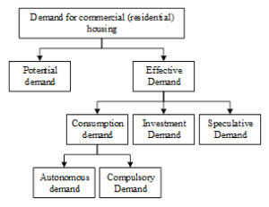
Demand for residential housing is the quantity of that type of commercial housing (residential) that consumers are willing and able to purchase at a given time and at a given price. Demand for commercial housing (dwellings) can also be divided into potential demand and effective demand based on the real ability to pay. According to the purpose of effective demand is divided into consumption demand and investment demand and speculative demand, of which consumption demand according to the subjective desire can be divided into autonomous demand and mandatory demand, residential demand classification as shown in Figure 1. Factors affecting the demand for housing market are multifaceted, mainly the following factors:
The level of national economic development
The level of demand for commercial housing and the level of national economic development into a positive relationship, its impact on the demand for commercial housing from two aspects: First, the scale of investment, the scale of investment is large, production operators are bound to increase the level of demand for factories, business houses, office buildings and so on. Second, the level of national income, the level of national income is the main variable governing personal disposable income, but also reflects the expansion of production capacity of enterprises is an important indicator, only the development of the economy, improve the level of national income, in order to make a city’s economy into a virtuous cycle, thereby constantly improving the productive demand for real estate and consumer demand. The growth of consumer demand is also a prerequisite for the formation of effective demand for commercial housing.
Level of urbanization
The city is the inevitable result of social and economic development, especially industrialization, the level of urbanization includes the expansion of the city scale and the growth of the urban population in two interrelated aspects, and the development of each aspect of the demand for commercial housing will increase. This is also a reflection of the real estate induced demand characteristics.
Consumer Income Level and Consumption Structure
The influence of consumer income level on the demand for commercial housing is divided into direct and indirect influence. The direct impact is mainly manifested in the demand for residential housing, which is basically a positive relationship. Indirect impact is mainly manifested in the increase in income level will promote the development of production, which in turn will expand the demand for productive real estate. Residents’ consumption structure on the impact of real estate is mainly manifested in the residents of the income of how much of the proportion spent on housing consumption, this proportion will have a direct impact on the purchasing power of housing commercialization after.
Due to the special characteristics of the real estate market leads to many market failure may, so the government’s intervention in the real estate market appears to be very inevitable and necessary, the government’s land policy, monetary policy and fiscal policy, etc. on the supply and demand for commercial housing will have a great impact on the policy factors naturally become one of the main factors in the fluctuation of commercial housing prices.
Land is the source of the development of commercial housing, the amount of land supply and the cost of land supply (e.g., the land premium and the way it is paid, the way the land is acquired) directly affects the supply of commercial housing, and an increase (or decrease) in the amount of land supply will result in a corresponding increase (or decrease) in the amount of commercial housing supplied. An increase (or decrease) in the cost of land supply will increase (or decrease) the price of commercial housing.
Monetary policy, such as interest rates, is a powerful lever for regulating the economy and has a greater constraint on productive and investment demand for real estate. Productive demand for real estate and investment demand can generally be viewed as an investment behavior, and thus higher interest rates, the demand for real estate has a dampening effect, lower interest rates, the demand for real estate has a role in promoting. The role of interest rates on real estate consumer demand is generally divided into two situations: one is the high and low changes in interest rates on loans to developers, resulting in changes in the price of commercial housing, thereby affecting the level of demand, and the second is the change in interest rates on loans to residents for personal housing, which will have a direct impact on the ability of consumers to pay, thereby affecting the level of their demand.
Generally speaking, the regulatory effect of fiscal and tax policies on the economy is indirect, and so is the impact on the real estate market. The analysis of fiscal and tax policies can be used to understand the changes in real estate development costs.
For example:
Financial policies adopted to stimulate the demand for housing, such as lowering interest rates, carrying out housing consumer credit, and implementing the housing provident fund system, all of which effectively increase the effective demand for housing.
Tax and fee reduction policies. In order to stimulate housing consumption, the authorities concerned have reduced taxes and fees on housing sales on several occasions.
In order to verify the influential relationship between socio-economic factors and house price volatility in the housing market, the SVAR model constructed in this study mainly includes the variables of residential price (HP), real gross domestic product (GDP), per capita disposable income (IV), real interest rate (RR), money supply (M), and exchange rate (ROE).
Real GDP:
Gross Domestic Product, or GDP, is the sum of all productive economic activities of a country or a region over a certain period of time. It is an important indicator reflecting the level of economic development of a country or a region, and can be viewed by direct search.
Per capita disposable income
The level of per capita disposable income is an important indicator of the purchasing power of the residents, and the level of the residents’ income determines the size of the purchasing power of the residents. Per capita disposable income (IV) = total income of residents – income tax – social security contributions – bookkeeping subsidies.
Real interest rate
The interest rate indicates the ratio of the amount of interest to the principal over a certain period of time. The level of the interest rate determines how much interest is earned on the principal over a certain period of time, and is based on the People’s Bank of China benchmark interest rate.
Money Supply
Money supply, refers to a country in a certain period of time for the social and economic operation of the money stock, that is, the potential and real purchasing power. Money supply (M) = cash in circulation outside banks + corporate and residential deposits + other deposits.
Exchange Rates
In today’s international market, there are two methods of expressing exchange rates, one is the indirect markup method, that is, a unit of national currency for how much foreign currency, and the other is the direct markup method, that is, a unit of foreign currency for how much national currency to the exchange rate of the foreign exchange bureau.
In this paper, quarterly data from 2014 to 2023 are selected to investigate the long-run dynamic relationship between house prices (HP) and real gross domestic product (GDP), disposable income per capita (IV), real interest rate (RR), money supply (M), and exchange rate (ROE). Since the raw data are a set of percentages, the data were first correlated before the empirical analysis. On the basis of taking logarithms of all the data, first-order differencing was carried out, so that a set of time-series data reflecting the changes in the real estate market was obtained.The GDP data per capita disposable income data were obtained from the database of the WI.com. The real interest rate is adopted from the one-year lending rate of the Central Bank. In the empirical analysis of this paper, since the data used are quarterly data, the impact of seasonal changes on economic development should be considered, so this paper uses econometric software to seasonally adjust each economic variable.
A structural vector autoregressive (SVAR) model was used to examine the dynamic influence mechanism between house price volatility and socio-economic factors in the housing market [22].
Consider a simplified form of a \(p\)st order VAR model: \[\label{GrindEQ__1_} X_{t} =\Gamma _{1} X_{t-1} +\Gamma _{2} X_{t-2} +\cdots +\Gamma _{p} X_{t-p} +u_{t} , \tag{1}\] where \(X_{t}\) is a \(k\)-dimensional vector, \(u_{t}\) is a \(k\)-dimensional disturbance term, and \(\Gamma\) is a matrix of parameters to be measured.
Because the VAR model has the defect of not being able to clarify the contemporaneous correlation between the variables in the system, it cannot identify the structural shocks. Therefore, the SVAR model relaxes the strict assumption of “zero contemporaneous effects between variables”, sets restrictive conditions based on relevant economic theories, decomposes the information of the model, and examines the contemporaneous relationship between each variable, and the SVAR model can be expressed as follows: \[\label{GrindEQ__2_} AX_{t} =\Gamma '_{1} X_{t-1} +\Gamma '_{2} X_{t-2} +\cdots +\Gamma '_{p} X_{t-p} +\varepsilon _{t} , \tag{2}\] \(\varepsilon _{t}\) is the white noise sequence and \(A\) is the contemporaneous relationship matrix between the variables. Left-multiplying both sides of Eq. (1) by matrix \(A\) yields: \[\label{GrindEQ__3_} AX_{t} =A\Gamma _{1} X_{t-1} +A\Gamma _{2} X_{t-2} +\cdots +A\Gamma _{p} X_{t-p} +Au_{t} . \tag{3}\]
Comparison of Eqs. (2) and (3) reveals that: \(Au_{t} =\varepsilon _{t}\) and further standard orthogonalization of \(\varepsilon _{t}\) yields: \(\varepsilon _{t} =Bv_{t}\), where \(E\left(v_{t} v'_{t} \right)=I_{k}\). The estimation of the SVAR model can then be expressed as: \[\label{GrindEQ__4_} Au_{t} =Bv_{t} . \tag{4}\]
In addition, \({k\left(k-1\right)\mathord{\left/ {\vphantom {k\left(k-1\right) 2}} \right. } 2}\) constraints need to be set on matrix \(A\) so that the SVAR model can be recognized and the relationships between the other coefficient matrices can be obtained accordingly.
In this paper, a SVAR model is constructed for six variables including residential prices (HP), real gross domestic product (GDP), disposable income per capita (IV), real interest rate (RR), money supply (M), and exchange rate (ROE). Assumption \(A_{0}\) is the lower triangular matrix, which is just identified using the recursive SVAR model. In this paper, the recursive shock transmission is set as:GDP\(\mathrm{\to}\)IV\(\mathrm{\to}\)M\(\mathrm{\to}\)RR\(\mathrm{\to}\)ROE\(\mathrm{\to}\)HP.The recursive SVAR model is set up as follows: \[\label{GrindEQ__5_} \left[\begin{array}{cccccc} {1} & {0} & {0} & {0} & {0} & {0} \\ {a_{21} } & {1} & {0} & {0} & {0} & {0} \\ {a_{31} } & {a_{32} } & {1} & {0} & {0} & {0} \\ {a_{41} } & {a_{42} } & {a_{43} } & {1} & {0} & {0} \\ {a_{51} } & {a_{52} } & {a_{53} } & {a_{54} } & {1} & {0} \\ {a_{61} } & {a_{62} } & {a_{63} } & {a_{64} } & {a_{65} } & {1} \end{array}\right]\left[\begin{array}{c} {e_{t}^{GDP} } \\ {e_{t}^{IV} } \\ {e_{t}^{M} } \\ {e_{t}^{RR} } \\ {e_{t}^{ROE} } \\ {e_{t}^{HP} } \end{array}\right]=\left[\begin{array}{cccccc} {b_{11} } & {0} & {0} & {0} & {0} & {0} \\ {0} & {b_{22} } & {0} & {0} & {0} & {0} \\ {0} & {0} & {b_{33} } & {0} & {0} & {0} \\ {0} & {0} & {0} & {b_{44} } & {0} & {0} \\ {0} & {0} & {0} & {0} & {b_{55} } & {0} \\ {0} & {0} & {0} & {0} & {0} & {b_{66} } \end{array}\right]\left[\begin{array}{c} {\hat{u}_{t}^{GDP} } \\ {\hat{u}_{t}^{IV} } \\ {\hat{u}_{t}^{M} } \\ {\hat{u}_{t}^{RR} } \\ {\hat{u}_{t}^{ROE} } \\ {\hat{u}_{t}^{HP} } \end{array}\right]. \tag{5}\]
To ensure the smoothness of the variables, the original absolute number variables were first logarithmized to eliminate possible time trends, and then the ADF method was used to test the smoothness of the variables. Except for Ln GDP and Ln IV, which are smooth series, all the other variables are non-smooth series, which are treated with first-order differencing. The results of the unit root ADF test for the variables are shown in Table 1. In the test form (C,T,K), C is the constant term, T is the time trend, K is the lag order, and the lag period is discriminated according to the AIC and SC information criterion. The ADF statistical test values of all unbalanced variables after treatment are -12.8864, -10.6659, -7.4929 and -8.8679, which are less than the critical values at 1%, 5% & 10% significance level, and they are all smooth series.
| Variable | Type | Statistics | 1% threshold | 5% threshold | 10% threshold | Conclusion |
| LnHP | (C,0,1) | -2.8751 | -4.1252 | -3.4411 | -3.1086 | Not smooth |
| DLnHP | (C,0,1) | -12.8864 | -4.0053 | -3.4621 | -3.1122 | Smoothness |
| LnRR | (C,0,1) | -1.5821 | -4.0793 | -3.4114 | -3.1622 | Not smooth |
| DLnRR | (C,0,1) | -10.6659 | -4.0831 | -3.4515 | -3.1613 | Smoothness |
| LnM | (C,0,1) | 0.4586 | -4.0791 | -3.4662 | -3.1559 | Not smooth |
| DLnM | (C,0,1) | -7.4929 | -4.0801 | -3.4681 | -3.1659 | Smoothness |
| LnROE | (C,0,1) | -3.5812 | -4.0172 | -3.4558 | -3.1601 | Not smooth |
| DLnROE | (C,0,1) | -8.8679 | -4.0781 | -3.4672 | -3.1612 | Smoothness |
The lag order of the SVAR model is determined by the lag order of the short-term VAR model. is the maximum lag order that reflects the interaction between variables. When the lag order is large enough, it can fully reflect the dynamic characteristics between variables. At the same time, the choice of lag order should take into account the number of observations. If the lag is too long, the parameters cannot be estimated correctly. Since the selected lag order affects the final estimation results of the vector autoregressive model, the optimal lag order of the model needs to be specified, and the results of the empirical test are shown in Table 2. The optimal lag order is shown in the rows where the corrected LR test statistic, the final prediction error, the Akaike informativeness, the Schwarz informativeness, and the Hannan-Quinn informativeness, and the rows where the most values with * are shown. The data in the table shows that there are four tests with an optimal lag order of order 5, which can be determined as the optimal lag order of the model.
| Lag | LogL | LR | FPE | AIC | SC | HQ |
| 0 | -102.24 | NA | 1.281E-5 | 2.623 | 3.484 | 3.519 |
| 1 | 367.572 | 864.462 | 7.623E-11 | -9.071 | -8.269 | -8.353 |
| 2 | 417.187 | 85.109 | 3.941E-11 | -9.345 | -7.527 | -9.716 |
| 3 | 535.191 | 185.2 | 3.225E-12 | -11.421 | -10.085 | -11.861 |
| 4 | 768.778 | 334.673 | 1.212E-14 | -18.692 | 14.244* | -16.423 |
| 5 | 808.772 | 51.675* | 8.635E-15* | -18.384* | -15.004 | -17.525* |
| 6 | 822.018 | 15.448 | 1.341E-14 | -17.823 | -13.376 | -15.591 |
| 7 | 844.079 | 21.882 | 1.744E-14 | -18.414 | -11.929 | -15.908 |
In this paper, the cointegration relationship of the above six variables is tested by using Johansen test [23]. The results of Johansen test are shown in Table 3.The trace statistic value of 36.882 is greater than the critical value of 29.553 at 5% level of significance and the statistic value of 24.659 is higher than the critical value of 20.852 at 5% level of significance. Therefore, there is at least one cointegration relationship with a confidence level of 95%.
| No null hypothesis of a co-integration relationship | Trace statistics | 5% threshold |
| Non-existent* | 36.882 | 29.553 |
| Maximum one* | 12.688* | 15.274 |
| Up to two | 4.759 | 3.711 |
| No null hypothesis of a co-integration relationship | \(\lambda\)-max statistics | 5% threshold |
| Non-existent* | 24.659 | 20.852 |
| Maximum one* | 7.389* | 14.033 |
| Up to two | 4.712 | 3.711 |
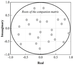
Then the overall smoothness of the model is tested, and the results of the overall smoothness test of the model are shown in Figure 2. The points of the inverse of the characteristic root modulus of the model are all within the unit circle, which indicates that the inverse of the characteristic polynomial roots of the constructed model are all less than 1, indicating that the structure of the SVAR(5) model is stable.
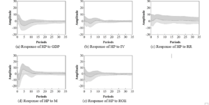
Finally, this paper finds that real gross domestic product (GDP), per capita disposable income (IV), real interest rate (RR), money supply (M), and exchange rate (ROE) have significant Granger effects on house price (HP) with through Granger causality test [24]. In order to further understand how each variable affects financial stability, impulse response analysis is conducted next, and the results of impulse response plots of different socioeconomic factors on house price volatility are shown in Figure 3. (a) (e) are the impulse responses of gross domestic product (GDP), per capita disposable income (IV), real interest rate (RR), money supply (M), and exchange rate (ROE) factors to the volatility of house prices, respectively. The impulse response function represents the impact on all endogenous factors when a shock of one standard deviation is applied to the error term in the model, which can graphically portray the dynamic transmission mechanism among the endogenous factors.
First, when facing a positive shock of one standard deviation of real gross domestic product (GDP), GDP produces a weak negative effect on house prices (HP), which shifts to a positive effect from period 3, and the effect of real GDP on the house price volatility index tends to zero from period 22 onwards. Second, in terms of disposable income per capita (IV), IV has a positive effect on house prices in the 1st period, continues to have a negative effect on house price volatility after the 5th period, and continues to have a negative effect until the 12th period, after which it tends to be zero. Again, looking at the real interest rate (RR), RR has a persistent positive effect on HP, which tends to zero after period 16. The exchange rate (ROE), on the other hand, has a positive effect on HP in period 1, which then becomes negative and increases, and the negative effect of exchange rate shocks on house price volatility lasts until period 12, after which it tends to zero, suggesting that although the rise in the RMB exchange rate can initially promote economic growth, in the long run it leads to expanding risks in the financial sector. Finally, in terms of money supply (M) M has a negative effect on HP at the beginning, and this negative shock reaches its highest level in period 2, after which the negative impact gradually diminishes and turns into a positive effect. Therefore, this paper finds that economic factors in the housing market can affect the volatility of China’s house prices in the short run, however, the impact of different economic policy choices of the government on China’s financial risk is long-lasting and strong.
| Period | GDP | IV | RR | M | ROE | HP |
| Phase 1 | 2.177 | 0.178 | 1.066 | 2.292 | 2.235 | 92.126 |
| Phase 2 | 2.088 | 5.122 | 2.048 | 2.231 | 3.456 | 88.714 |
| Phase 3 | 1.959 | 10.269 | 3.115 | 2.312 | 4.523 | 74.323 |
| Phase 4 | 1.684 | 12.887 | 4.243 | 2.411 | 5.985 | 70.502 |
| Phase 5 | 1.487 | 15.783 | 5.147 | 7.464 | 7.303 | 67.773 |
| Phase 6 | 1.523 | 17.345 | 5.255 | 7.478 | 7.106 | 63.229 |
| Phase 7 | 1.689 | 18.694 | 6.278 | 7.479 | 7.098 | 61.053 |
| Phase 8 | 1.711 | 19.213 | 7.153 | 6.985 | 7.055 | 59.227 |
| Phase 9 | 1.942 | 21.087 | 7.824 | 6.059 | 7.001 | 57.412 |
| Phase 10 | 2.058 | 22.913 | 8.159 | 5.791 | 6.943 | 56.335 |
| Phase 11 | 2.012 | 22.926 | 8.193 | 5.612 | 6.912 | 56.001 |
| Phase 12 | 2.151 | 23.015 | 8.241 | 5.587 | 6.899 | 55.992 |
| Phase 13 | 2.223 | 23.018 | 8.305 | 5.498 | 6.875 | 55.876 |
| Phase 14 | 2.033 | 23.112 | 8.382 | 4.982 | 6.666 | 55.655 |
| Phase 15 | 2.069 | 23.221 | 8.494 | 4.267 | 6.651 | 55.498 |
In order to further analyze the degree of the role of socio-economic factors on house price volatility (HP) in the housing market, so as to reflect the impact of each economic factor on the stability of house prices, this paper carries out the variance decomposition, and the results of the variance decomposition of each factor on HP are shown in Table 4. The variance decomposition can accurately show the contribution value of unit variance shock to the change of each endogenous variable. 15 periods of variance decomposition effect of house price volatility is mainly affected by itself and residents’ disposable income, the degree of explanation of its volatility is 55.5% and 23.2%, respectively, and the real interest rate (RR), the exchange rate (ROE) and the money supply (M) are next to the real interest rate (RR) and the exchange rate exceeded the influence of money supply on the house price after period 8, while the real GDP and money supply have more impacts on house price than money supply, while real GDP has more impacts on house price. House prices, while real GDP has the lowest impact on house prices. The influence of money supply and interest rate on house price decreases year by year, and the rapid increase of house price is not conducive to the healthy economic development of the city.
This paper collects and organizes economic statistics of real GDP, disposable income per capita, real interest rate, money supply and exchange rate and house price from the first quarter of 2014 to the first quarter of 2023, and constructs a structural vector autoregressive SVAR model. House price fluctuations are mainly affected by itself and disposable income per capita, with an explanation degree of 55.5% and 23.2% respectively, followed by real interest rate (RR), exchange rate (ROE) and money supply (M), and the exchange rate exceeds the effect of money supply on house prices after period 8, while real GDP has the lowest effect on house prices. The influence of money supply and interest rate on house price decreases year by year, and the rapid increase of house price is not conducive to the benign economic development of the city. This paper finds that economic factors in the housing market can have an impact on the volatility of house prices in China in the short term, however, the impact of different economic policy choices of the government on China’s financial risk is long-lasting and strong. Therefore, the following policy recommendations are proposed:
To control real estate prices, it is necessary to make interest rates as stable as possible within a reasonable range, not to make substantial adjustments to interest rates, and at the same time to make a good correlation between related financial and monetary policies. At the same time must first stabilize the exchange rate of the RMB, even if the RMB is to be appreciated, but the magnitude of RMB appreciation in a short period of time should not be too large.
For different situations, different policies should be implemented. Due to the imbalance of economic development between regions, there are great differences in real estate prices between cities in various regions. Therefore, the government should implement differentiated policies for the actual situation of real estate prices in different regions.
Focus on the linkage between the regulation of the housing market and the macroeconomy, and do a good job of long-term planning for the real estate market. To prevent the real estate market adjustment speed is too fast to the development of the macro economy to bring too many negative effects. In addition, in the process of promoting the reform of the housing system, it is also necessary to pay attention to the construction of policy-guaranteed housing, and to maintain a reasonable volume-ratio relationship between the two.