1. Introduction
With the continuous penetration and development of society, medicine, and the elderly environment, the problem of population aging is gradually emerging. It can be seen from Table 1 that the growth rate of the elderly population in my country will exceed 8 million per year, and it is expected to continue to grow by 20.3% from 2020 to 2050. The aging of the population will accompany the 21st century [1]. Today, the problem of aging in our country has become a major social issue of increasing concern, and it is also an issue that every family needs to discuss more and more. In China, the research on the practice of living space for the elderly is relatively late.
Affected by modern factors such as average life expectancy, rapid urbanization, and a severe shortage of labor in the future, the traditional family pension model has become increasingly weakened with social development, and changes in the structure of family members have become increasingly weak. Obviously cannot meet the various elderly needs of the elderly. With the help of the home based care between the society and the family, more attention is paid to it, and it is more worthy of discussion to be accepted by the elderly in a non disabled state. Faced with the reality of alleviating the shortage of nursing beds in institutional nursing homes and social nursing homes [2].
For example, with the physical and psychological changes such as vision and grip strength of the elderly, living alone in a room that is too empty, a sense of worthlessness due to a decline in social status, nervousness up and down stairs, walking on smooth ground in the passage area, and lack of refined design, etc. From this, it is necessary to study the traditional filial piety culture, the behavior of the elderly, and the spatial adaptability of the elderly in my country’s urban elderly [3–4]. This further shows that the 60-year-old does not mean old age. The research of this project is the adaptive research of the space design for the elderly in the period of independent survival of the elderly, that is, in the non-disabled state. The distinctive feature of design theory research was that it revolved around the expanding functional model and social needs, around the evolution of the environment, and took the form of multidisciplinary systematization, from the modernist trend of humanized design to humanized housing.
The theory of design is an eternal research topic, and with the progress of people’s cognition, technology and culture, there will be newer cognition and understanding [5]. The continuous deepening of high-tech, Internet, and smart home has brought new opportunities for the elderly-friendly design in the elderly space. Through the Internet, technology can be used to break the ice for home care, providing scientific support for improving the quality of life of the elderly. Today, the adaptability, scientific Ty and epochally of the design suitable for the elderly in urban high-rise residential buildings are the worthiest of discussion at present in the elderly space and home care model.
| particular year | 2020 | 2025 | 2030 | 2035 | 2040 | 2045 | 2050 |
|---|---|---|---|---|---|---|---|
| Total population (100 million) | 13.98 | 13.94 | 13.78 | 13.52 | 13.15 | 12.67 | 12.11 |
| Population over 60 years old (100 million) | 2.43 | 2.90 | 3.47 | 3.91 | 4.04 | 4.19 | 4.55 |
| Proportion of elderly population (%) | 17.31 | 20.81 | 25.11 | 29.91 | 30.61 | 33.02 | 37.61 |
In recent years, with the rise of deep learning and the development of data-driven networks, researchers have begun to use deep neural networks for feature extraction and perception of TM sequences. Deep learning is good at dealing with nonlinear problems and is widely used in TM prediction [6]. For example, [7] utilizes a deep belief network that utilizes stacked autoencoders. and its variant long short-term memory model and gated cyclic unit adopt sequential structure and have a certain time memory function and are widely used by researchers in traffic forecasting. Better prediction results. [8] conducted a comprehensive test on the deep learning-based TM prediction, and the experimental results show that among the existing deep learning methods, RNN and its variants have higher prediction accuracy than SAE and DBN. However, the RNN-based model from the beginning to the end, only the time series features are considered, and the spatial features are ignored. In order to better describe the spatial features, some studies have introduced convolutional neural networks to model the space [9].
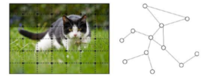
Taking image data as an example, as shown in Figure 1, a picture can be represented as a set of rules in Euclidean space. For scattered pixels, translation invariance means that with any pixel as the center, the local structure of the same size can be obtained, while the data of the graph structure has no translation invariance. The convolutional neural network learns the volume shared by each pixel. Accumulate kernels to model local connections, and then learn meaningful hidden layer representations for pictures. Computer networks are essentially represented by graph data [10]. However, inspired by CNN, with the help of convolutional neural networks, the ability to model local structures and the ubiquitous node dependence on graphs Relational, his characteristic of graph convolutional network makes it have unique advantages in processing graph-structured data. In recent years, graph convolutional network has made great achievements in text classification, network analysis, traffic prediction and other fields. develop.
Based on this, this paper proposes a new neural network model graph convolution gated recurrent unit, which can capture the temporal and spatial characteristics of complex traffic data, deploy it on the SDN controller, and can be used for traffic prediction based on SDN network [11].
2. Proposed Methods
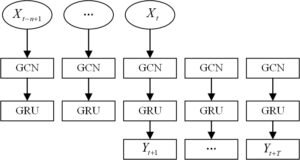
We use \(G = \left( {V,E} \right)\) describe the topology of the graph, each network node is a vertex, \(V\) represents the set of vertices \(V = \left\{ {{V_1},{V_2},…{V_N}} \right\}\), \(E\) is the edge of the graph \(A\) set. \(A\) represents the adjacency matrix of the graph \(G\), \(D\) represents the degree matrix of the graph \(D \in {R_N} \times NX\). We regard the network traffic matrix \(X\) as the feature of the vertex, as shown in Figure 2, \(X_t\) represents the time \(t\) Eigen matrix \(X \in {R_N} \times N\).

Therefore, a mapping function \(f\) based on the topological graph \(G\) and the feature matrix \(X\), namely:
\[\label{e1} \left[ {{X_{t + 1}},…,{X_{T + 1}}} \right] = f\left( {G,{X_{t – m + 1}},…,{X_t}} \right)\tag{1}\] where, \(T\) represents the length of the output prediction sequence. Due to the lack of translation invariance on the graph, it is difficult to define a convolutional neural network in the node domain [12]. The Fourier transform of the signal convolution is equivalent to the product of the signal Fourier transform:
\[\label{e2} F\left( {f*g} \right) = F\left( f \right)*F\left( g \right)\tag{2}\]
Where, \(g\) represent the original signals, \(F\left( f \right)\) represents the Fourier transform of \(f\), \(*\) represents the convolution operator. Perform the inverse Fourier transform on both sides of Eq. (1), we can get:
\[\label{e3} f*g = {F^{ – 1}}\left( {F\left( f \right)*F\left( g \right)} \right)\tag{3}\]
Taking the eigenvectors as a set of bases in the spectral space, the Fourier transform of the signal \(X\) on the graph is:
\[\label{e4} \mathop x\limits^ \wedge = {U^T}x\tag{4}\]
Among them, \(x\) refers to the original representation of the signal in the node domain; \(\mathop x\) refers to the representation of the signal \(x\) transformed to the spectral domain; \({U^T}\) represents the transpose of the eigenvector matrix for Fourier transform. Since \({U}\) is a positive definite matrix, the signal \(x\) is the inverse Fourier transform can be expressed as:
\[\label{e5} x = {\left( {{U^T}} \right)^{ – 1}}\mathop x\limits^ \wedge = U\mathop x\limits^ \wedge\tag{5}\]
Using the Fourier transform and inverse transform on the graph, we can implement the graph convolution operator based on the convolution theorem:
\[\label{e6} x*Gy = U\left( {{U^T}x} \right)\Theta \left( {{U^T}y} \right)\tag{6}\]
We use a diagonal matrix \({g_\theta }\) to replace the vector \({U^T}y\), Then Hadamard multiplication can be transformed into matrix multiplication. Graph convolution can be expressed as follows:
\[\label{e7} x*Gy = U{g_\theta }{U^T}x\tag{7}\]
In Eq. (7), \({g_\theta }\) is the convolution kernel to be learned, and in spectral convolutional neural networks, \({g_\theta }\) is in the form of a diagonal matrix, and there are \(n\) parameters to learn [13]. The Chebyshev network parameterizes the convolution kernel \({g_\theta }\):
\[\label{e8} {g_\theta } \approx \sum\limits_{i = 0}^{K – 1} {{\theta _k}} {T_k}\left( {\mathop \Lambda \limits^\Lambda } \right)\tag{8}\]
A) Model Structure
The GCN model has two parts: GCN and GRU. As shown in Figure 3, we use the time series data of n historical moments as input according to Eq. (1), and the graph convolution network extracts the network topology to obtain spatial features, and then uses the he time series with spatial features is put into the GRU, the dynamic changes are captured through the transfer of information between units, and the temporal features are extracted; finally, it is sent to the fully connected layer to output the prediction result [14–15].
1) Modeling Spatial Features
Obtaining complex spatial features is a key problem in network traffic prediction. Traditional CNN is only suitable for Euclidean space, network topology is not a grid, but CNN cannot handle data of complex topology type. GCN can handle graph structure, which has been widely used Applied to document classification and image classification [16]. GCN builds filters in the Fourier domain, acts on vertices and their first-order neighborhoods, and extracts spatial features between vertices. As shown in Figure 4, it is assumed that vertex 1 is in the network. According to Eq. (9), the mathematical expression of the GCN layer is:
\[\label{e9} {X^{(m + 1)}} = \operatorname{ReLU} \left( {{{\hat D}^{ – 1/2}}\hat A{{\hat D}^{ – 1/2}}{X^{(m)}}{W^{(m)}}} \right)\tag{9}\]
.

2) Modeling temporal features
RNN can reflect long-distance dependency information when processing sequence data including recordings and texts. Connections are established between RNN layers and neurons, and the state of the current moment can affect the state of the next moment, so it can be captured. Before and after correlation of data. GRU designs a gated structure based on RNN, allowing information to be selectively transmitted in the hidden layer, memorizing important information and solving the problems of gradient disappearance and gradient explosion in the process of long sequence training. GRU has There are two gated structures, reset gate and update gate, with few parameters and fast convergence speed [17–18]. The transmission between states in GRU is a one-way propagation process from front to back, and only the current input and previous context information can be used, as shown in Figure 5. When capturing the traffic information at the current moment, the model still retains historical information and could extract temporal features.

3) Modeling by combining temporal and spatial features
To extract spatial and temporal features at the same time, we combine GC and GRU, first use GC to extract spatial features, and then use GRU to extract spatial features [16–17], the mathematical expression is as follows:
\[\label{e10} \begin{aligned} & u_t=\sigma\left(W_u\left[f\left(A, X_t\right), h_{t-1}\right]+b_u\right) \\ & r_t=\sigma\left(W_r\left[f\left(A, X_t\right), h_{t-1}\right]+b_r\right) \\ & c_t=\tanh \left(W_c\left[f\left(A, X_t\right), r_t * h_{t-1}\right]+b_c\right) \\ & h_t=u_t^* h_{t-1}+\left(1-u_t\right) * c_t \end{aligned}\tag{10}\]
where \(f\left( {A,{X_t}} \right)\) represents the graph convolution process, and \(W\) and \(b\) represent the trainable parameters of the GRU in Section 2.
4) Loss function
During training, the goal is to minimize the squared difference between the true value of the error flow and the predicted value of the flow. We denote the true value of the flow and the predicted value of the flow by \({Y_t}\) hand \({Y_{\Lambda t}}\). To prevent overfitting, the regularization term \({L_2}\) is added, where \(\lambda\) is a hyperparameter. The formula of the loss function is as follows:
\[\label{e11} Loss = |{Y_t} – {\mathop Y\limits^\Lambda _t}{|^2} + \lambda {L_2}\tag{11}\]
3. Experimental Results and Analysis
Table 2 lists the prediction results of the GCGRU model and other baseline methods at 15min, 30min, and 45min. The GCGRU model obtains the best prediction performance among all evaluation indicators, which proves that GCGRU has better performance in space and time. Prediction ability. It can also be found in Table 2 that methods based on neural networks, including GCGRU model, GRU model, etc., which emphasize the extraction of time series features, usually have better prediction performance than other baselines, such as SVR model and ARIMA model. The prediction results of the network in 15min are shown in Figure 6 and 7. In the 15min traffic prediction task, The RMSE error of GCGRU is about 8.2% lower than that of GRU model, and the accuracy rate is about 17% higher than that of GRU. The prediction effect of ARIMA and SVR is the worst, mainly because the linear method is difficult to deal with complex and non-stationary time series. Data. The poor prediction effect of GCN model is because GCN considers spatial characteristics and ignores traffic data, which is typical time series data.
| Algorithm | RMSE (15 min/30 min/45 min) | MAE (15 min/30 min/45 min) | MAPE (15 min/30 min/45 min) |
|---|---|---|---|
| ARIMA | 0.52916/0.52908/0.52906 | 0.43978/0.43974/0.43969 | 7.3917/7.3826/7.3844 |
| SVR | 0.10145/0.101168/0.10164 | 0.08391/0.08452/0.08479 | 10.9375/10.9934/11.0113 |
| FCNN | 0.02798/0.03089/0.03214 | 0.02055/0.02234/0.02512 | 2.8921/3.1346/3.4002 |
| GCN | 0.02666/0.02864/0.03018 | 0.02027/0.02188/0.02516 | 3.0057/3.3014/3.5125 |
| GRU | 0.01997/0.02156/0.02384 | 0.01487/0.01628/0.01826 | 1.8687/2.01536/2.2578 |
| GCGRU | 0.01739/0.01902/0.02124 | 0.01232/0.01433/0.01598 | 1.5409/1.7274/2.1033 |
Figure 8 compares the prediction effects of GCGRU, GCN and GRU. For example, in the 15min flow prediction, the RMSE of the GCGRU model is reduced by about 35.6% compared with the GCN model; in the 30min flow prediction, the GCGRU model is comparable to the GCN model. Compared with the GRU model, the RMSE is reduced by about 33.6%, indicating that the GCGRU model can effectively extract spatial features. In the 15min flow prediction, the GCGRU model reduces the RMSE by about 9.5% compared with the GRU model; in the 30min flow prediction, the RMSE is reduced by about 9.5%. compared with the GCN model, the RMSE of the GCGRU model is reduced by about 13.0%, which indicates that the GCGRU model can effectively extract temporal features.
Figure 9 shows the prediction effect of the GCGRU model for 15min, 30min and 45min respectively. With the extension of the prediction task, the error of the GCGRU model also increases, but the prediction effect is basically sTable Therefore, the GCGRU model can not only be used for short-term traffic It can also be used for medium and long-term forecasting, but it still does not perform well in the forecasting of peak traffic.

4. Conclusion
This study proposes an improved graph convolution deep neural network (GCGRU) algorithm for the ageing design problem of urban living space environment under the background of aging. This algorithm can effectively mine out the existing graph convolution algorithms. The spatial-temporal dependence of complex networks. This research has carried out large-scale experiments and verification work on the GEANT dataset. The results show that, compared with other classical algorithms, GCGRU’s future improvement in prediction accuracy is mainly as follows: 1) Continue to explore how to improve the interpretability of the deep learning algorithm, and try to find the causal relationship that the model has good prediction accuracy; 2) Since only the 1st-order network neighborhood is extracted, some neighbor information may be missed. For this reason, further research will include more neighbors. 3) There is only traffic matrix at each moment in the data set as a feature, and more features such as link bandwidth can be considered; 4) It can be combined with other models, such as reinforcement learning, to explore more application scenarios.