1. Introduction
The emerging technology represented by Internet technology is the most widely used and mature innovation technology at present, which has also given rise to a series of new economic forms such as the Internet economy or digital economy [1–2]. Under the urgent need of realistic development and corresponding policy guidance, China’s digital economy is developing rapidly, playing an important role in stimulating consumption, boosting investment, creating employment, enhancing innovation and competitiveness, and providing a new dynamic energy and feasible path for promoting China’s high-quality economic development and building a modern economic system.
In recent years, researchers have improved forecasting outcomes by using econometric and machine learning methods to forecast financial time series data. However, deep learning employs unsupervised learning of layer-by-layer feature extraction, which has more potent feature representation capabilities and can learn more complex function representations than machine learning and econometric techniques. Deep learning also has stronger generalization capabilities, is more likely to reduce overfitting issues while increasing the prediction accuracy of in-sample data, and is better able to depict the long-memory nature of time series thanks to algorithms like long short-term memory neural networks (LSTM) [3–4]. Deep learning is therefore more suited to financial time series data prediction with complicated features.
There is no direct evidence on the actual role of the rapid development of the digital economy in building a modern economic system, which may result in narrowing or exaggerating the role of technologies such as the Internet in the economy, further leading to bias in policy making. In turn, the acquisition of direct evidence is faced with a series of problems such as poorly defined concepts, lagging statistics and lack of measurement methods [5]. Therefore, one of the feasible ways to solve this problem is to clarify the intrinsic mechanism and practical role of the digital economy in promoting high-quality economic development from a theoretical perspective. The causes influencing changes in financial time series data over the short, medium, and long periods are complicated and varied. Researchers have suggested combining wavelet analysis, empirical modal decomposition (EMD), and integrated empirical modal decomposition (EEMD) to create a combined prediction approach for financial time series data in order to increase forecast accuracy [6]. The drawback of harmonics without a clear physical meaning that easily occurs in wavelet analysis can be overcome by EEMD, which can extract the components and trends of time series data in an adaptive manner [7].
The forecasting approach in this study has the following benefits over current forecasting models for financial time series data: First, CNN-GRU neural networks have extensive feature extraction capabilities and can effectively capture complicated links among financial time series data, such as non-linear and non-smooth interactions. This is in contrast to typical econometric models and machine learning methods [8]. Second, when compared to recurrent neural networks like GRU, CNN-GRU neural networks can incorporate local spatial correlation features of financial time series data, allowing the interrelated features of various financial time series data to be fully taken into account. Additionally, when compared to CNN, CNN-GRU neural networks can better handle both long-term and short-term serial dependence features. Thirdly, there are three aspects that can be used to build financial time series forecasting models: short-term disruptions, medium-term cycles, and long-term trends. Time series data forecasting models can be built using various frequencies and volatility characteristics [9–11]
2. MF-DCCA
The high-dimensional multifractal behavior between two time series is mostly calculated using the MF-DCCA approach, which was first proposed in [12–15]. Later, it was successfully employed to investigate the connections between crude oil and freight index, as well as the Chinese gold market and trading volume. In order to analyze the cross-correlation and multifractal properties between two time-series variables, MF-DCCA is primarily used, MF-DCCA as shown in Figure 1. The method is effective at removing the impact of local trends in the series on the series and can be used to observe the multifractal behavior of the time series at various time scales.

Where, \(x\left( t \right)\) and \(y\left( t \right)\) denote two time series,\(t = 1,2, \ldots ,N\), respectively, where \(N\) denotes the length of the time series. Figure 1 illustrates the computational flow of MF-DCCA, which is divided into the following steps, as follows:
Step 1: Construct two new time series variables based on \(x\left( t \right)\) and \(y\left( t \right)\), where \(\bar x\) and \(\bar y\) are the corresponding mean values.
Step 2: Divide the reconstructed sequences \(X(t)\) and \(Y(t)\). For each given time window \(s\), \(2N_s\) non-overlapping time windows can be obtained.
Step 3: The local trend functions \({x_\lambda }\) and \({y_\lambda }\) are obtained by fitting the time series with a window of \({\lambda }\) for each window using least squares. The original time series is then differenced from the local trend function to eliminate the trend for each time window, and the local covariance function is calculated [14–15].
Step 4: The \(q\) order wave function can be obtained by averaging the local covariance over \(2{N_s}\) windows. When \(q = 2\), MF-DCCA is equivalent to MF-DFA.
\[\label{e1} {F_0}(s) = \left\{ {\frac{1}{{4{N_s}}}\sum\limits_{\lambda = 1}^{2{N_s}} {\left[ {\ln {F^2}(s,\lambda )} \right]} } \right\}q = 0\tag{1}\]
A. Time Series Decomposition Algorithm
A time series is broken down into three variables using STL, which is based on the LOESS smoother. Stable and ordered subsequences following data decomposition can highlight the data features, and pre-processing the data utilizing STL decomposition techniques can reduce the uncertainty brought on by data noise [16]. STL is more resistant to time series outliers and easier to apply than decomposition methods like wavelet transform and empirical modal decomposition, and it can be used for the majority of time series decomposition [17–18].
Denoting the time series to be decomposed by \({X_t}\), STL can decompose it into trend component \(\left( {{T_t}} \right)\), seasonal component \(\left( {{S_t}} \right)\) and residual component \(\left( {{R_t}} \right)\), and the result of the decomposition satisfies Eq. (2).
\[\label{e2} {X_t} = {S_t} + {T_t} + {R_t}\tag{2}\]
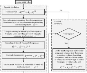
The computational process of the STL algorithm consists of two processes. Suppose \(S_t^{\left( k \right)}\) and \(T_t^{\left( k \right)}\) are the seasonal and trend components at the end of the kth iteration process of the inner loop, and \(S_t^{\left( k+1 \right)}\) and \(T_t^{\left( k+1 \right)}\) at the update of the \(k+1\)th iteration, initially \(T_t^{\left( k \right)} = 0\). The computational flow chart of the STL algorithm is shown in Figure 2, and the specific computational process is divided into the following steps.
Step 1: Detrending
\[\label{e3} X_t^{trend} = {X_t} – T_t^{\left( k \right)}\tag{3}\]
Step 2: Periodic subsequence smoothing. Apply the Loess smoother to each periodic subsequence to obtain the initial seasonal sequence \(C_t^{\left( {k + 1} \right)}\).
\[\label{e4} S_t^{\left( {k + 1} \right)} = C_t^{\left( {k + 1} \right)} – L_t^{\left( {k + 1} \right)}\tag{4}\]
Step 3: Remove seasonal items. A nonseasonal step was calculated.
\[\label{e5} X_t^{deseason} = {X_t} – S_t^{\left( {k + 1} \right)}\tag{5}\]
When the seasonal and trend components are updated in the next iteration, the weights are used to reduce the effect of the outliers.
\[\label{e6} R_t^{\left( {k + 1} \right)} = {X_t} – T_t^{\left( {k + 1} \right)} – S_t^{\left( {k + 1} \right)}\tag{6}\]
B. Complexity analysis theory
The R/S method is an effective statistical indicator for quantitatively portraying the long-term dependence of time-series data, where long-term dependence is mainly reflected in the self-similarity process of time-series data [19]. Most natural phenomena have self-similarity, such as temperature, rainfall and humidity. In addition to studying the dynamics of such natural phenomena, the method has also been used in the analysis of stock and exchange rate markets, where the R/S analysis is calculated as follows:
Slice the time series \(x\left( t \right)\) into \(L\) consecutive subseries of length \(n\). Each subseries is denoted \({I_a}\), \(a = 1,2,…,m\). The elements in \({I_a}\) are denoted \(E\left( {k,m} \right),k = 1,2,…,n,m = 1,2,…,L\). Calculate the cumulative deviation of all subsequences:
\[\label{e7} {R_{{I_\alpha }}} = \max (X(k,\alpha )) – \min (X(k,\alpha ))\tag{7}\]
The standard deviations are
\[\label{e8} S_{{I_\alpha }} = {\left[ {\frac{1}{n}\sum\limits_{i = 1}^n {{{\left( {E(k,\alpha ) – {{\bar I}_\alpha }} \right)}^2}} } \right]^{\frac{1}{2}}}\tag{8}\]
According to Eq. (7) and (8), the rescaled polar differences are expressed as
\[\label{e9} {(R/S)_n} = \frac{1}{L}\sum\limits_{\alpha = 1}^L {\frac{{{R_{{I_\alpha }}}}}{{{S_{{I_\alpha }}}}}}\tag{9}\]
The Hurst index is related to the re-scaled extreme deviation as:
\[\label{e10} {(R/S)_n} = {(an)^{{\text{Hurst }}}}\tag{10}\]
Where \({a}\) is a constant and \({Hurst}\) is known as the Hurst exponent. When \(Hurst=0.5\), it means that the time series is random, there is no long-range correlation, and the increment in past time is independent of the increment in future time. When \(0<Hurst<0.5\), it means that the time series variable has negative long-range correlation, i.e. if the trend was up in the past, then there is a high probability that the trend will reverse in the future, i.e. the trend will be down. Conversely, if the past is a downward trend, there is a high probability that the future will show an upward trend. When \(0.5<Hurst<1\), the time series variables have a positive long-range correlation, meaning that past and future are likely to have the same trend, with the probability of this increasing the closer is to 1. Although the index calculated by the R/S method has the same interpretation as the Hurst finger data calculated by MF-DCCA, the R/S method is applied to calculate the similarity of the time-series variables themselves, whereas MF-DCCA calculates the similarity and multifractality between two time-series variables [20].
3. Empirical Investigation
The feasibility of applying CNN-GRU neural networks to financial time series data forecasting is theoretically explored, and the basic principle of EEMD decomposition of financial time series data is analyzed [21]. Taking the SSE index as an example, the practical effects of applying CNN-GRU neural networks to financial time series data forecasting are empirically explored to compare the effects of integrated forecasting of financial time series data with those of direct forecasting. It should be noted that the selection of activation functions for different training models is mainly determined by the performance of the models in the training and validation sets, while the number of hidden units and penalty term parameters in the neural network layers are determined by grid search.
A. Feature vector selection and data description
The sample data were taken from the Wind database and ranged from 2011/01/01 to 2018/12/01. The sample data were divided into three sets: a training set, a validation set, and a test set. The training set was used to train the neural network parameters, the validation set to validate the neural network model, the test set to validate the neural network structure, and the test set to evaluate the prediction and generalization capabilities of the EEMD-CNN-GRU neural network model, as shown in Table 1.
| Data Transaction | Days | Time |
|---|---|---|
| Training Set | 1540 | 2011/01/04-2017/05/09 |
| Verification Set | 193 | 2017/05/10-2018/02/13 |
| Test Set | 194 | 2018/02/14-2018/12/01 |
Taking into account the existing research literature and data availability, and fully considering the impact of different financial markets on the SSE, the following eigenvectors are selected to construct a prediction model for the closing price of the SSE, as shown in Table 2.
| Feature vector | Index | Feature vector | Index |
|---|---|---|---|
| \({x_1}\) | Yesterday’s closing price of the Dow Jones Industrial Average | \({x_{11}}\) | 5-day average trading volume |
| \({x_2}\) | Yesterday’s closing price of the S&P 500 | \({x_{12}}\) | 20 day average trading volume |
| \({x_3}\) | Hang Seng Index closing price yesterday | \({x_{13}}\) | 5 day moving average |
| \({x_4}\) | Yesterday’s closing price of the European Stoxx 50 index | \({x_{14}}\) | 20 day moving average |
| \({x_5}\) | Yesterday’s closing price of the Nikkei 225 index | \({x_{15}}\) | 12 day moving average index |
| \({x_6}\) | Yesterday’s closing price | \({x_{16}}\) | Exponential Smoothing Moving Average |
| \({x_7}\) | Yesterday’s opening price | \({x_{17}}\) | Relative strength index |
| \({x_8}\) | Yesterday’s highest price | \({x_{18}}\) | Trend indicators |
| \({x_9}\) | Yesterday’s lowest price | \({x_{19}}\) | Volume ratio |
| \({x_{10}}\) | Yesterday’s trading volume |
B. EEMD Decomposition and IMF Reconstruction
The SSE index can be broken down into 14 IMF components and one residual component using the EEMD decomposition. According to Figure 3, the IMF1 to IMF14 components and the residual component RES display the SSE index’s volatility characteristics at various time scales, from high frequency to low frequency, respectively.
Figure 3 shows that the frequency of fluctuations gradually decreases from the IMF1 component to the IMF14 component, with the IMF1 IMF6 component having a higher frequency, smaller amplitude, and a relatively greater degree of volatility, reflecting the short-term sharp fluctuations and specifics of the SSE index fluctuations. The IMF7–IMF14 component shows less information about the volatility of the index but has a lower frequency, greater amplitude, and a substantially lower degree of volatility. It reflects medium–long term patterns. The residual RES component depicts the SSE index’s overall long-term trend. Further provided in three dimensions, including correlation coefficient, variance contribution ratio, and number of trips, the link between the IMF component, RES residual term, and SSE index is illustrated in Table 3.

The degree of association between the elements broken down by EEMD and the SSE index is indicated by the correlation coefficient. The correlation coefficients between the IMF1 through IMF4 components and the SSE index are all less than 0.1, as shown in Table 3. The IMF1 IMF9 components and the SSE index have relatively low correlations, as shown by the IMF5 IMF9 components’ correlation coefficients, which are all in the range of 0.1 0.2. The correlation coefficients of the IMF10-IMF14 components and the residual RES component are all greater than 0.3, indicating that the correlation between these components and the SSE index is relatively high. 3, indicating that these components have a relatively high correlation with the SSE. Thus, from the correlation coefficients, it is clear that sharp short-term fluctuations have a relatively small impact on the SSE Index, while changes in trends in the medium to long-term range have a relatively large impact on changes in the SSE Index.
| Modality | Correlation coefficient | Number of runs | Modality | Correlation coefficient | Number of runs |
|---|---|---|---|---|---|
| IMF1 | 0.0205 | 1298 | IMF9 | 0.1692 | 20 |
| IMF2 | 0.0256 | 782 | IMF10 | 0.3943 | 10 |
| IMF3 | 0.0455 | 474 | IMF11 | 0.4753 | 8 |
| IMF4 | 0.0780 | 282 | IMF12 | 0.6782 | 6 |
| IMF5 | 0.1122 | 170 | IMF13 | 0.8473 | 2 |
| IMF6 | 0.1128 | 94 | IMF14 | 0.7838 | 2 |
| IMF7 | 0.1727 | 53 | RES | 0.6416 | – |
| IMF8 | 0.1896 | 39 |
The IMF components are reconstructed into high-frequency and low-frequency components by using travel codes, and the travel numbers of each IMF component are shown in Table 3. The travel numbers of IMF1-IMF6 are larger, indicating that these IMF components are more volatile, while the travel numbers of IMF7 to IMF14 are smaller and gradually decreasing, indicating that these components are less volatile. Setting 90 as the threshold for high-frequency components, IMF components with a range greater than 90 are reconstructed as high-frequency components, reflecting short-term stochastic perturbations in the SSE, while IMF components with a range less than 90 are reconstructed as low-frequency components, reflecting medium-term events affecting the SSE. Therefore, IMF1-IMF6 are reconstructed as high-frequency components, IMF7-IMF14 are reconstructed as low-frequency components, and the residual term RES is the long-term trend term.
C. Exploring the effect of direct prediction
In order to explore the practical effect of CNN-GRU neural networks in financial time series data, CNN, GRU neural networks, LSTM and machine learning such as BP neural networks (BPNN), SVM on the direct prediction effect of the undecomposed SSE index. For the prediction accuracy of the model, the Theil inequality coefficient and MAPE were used to measure the expressions as:
\[\label{e13} {\text{Theil }} = \sqrt {1/T\sum\limits_{t = 1}^T {{{\left( {Y_t^{{\text{pre }}} – Y_t^{{\text{true }}}} \right)}^2}} /} \left( {\sqrt {1/T\sum\limits_{t = 1}^T {{{\left( {Y_t^{{\text{pre }}}} \right)}^2}} } + \sqrt {1/T\sum\limits_{t = 1}^T {{{\left( {Y_t^{{\text{true }}}} \right)}^2}} } } \right)\tag{11}\]
\[\label{e14} {\text{ MAPE }} = 1/T\sum\limits_{t = 1}^T {\left| {\frac{{Y_t^{{\text{pre }}} – Y_t^{{\text{true }}}}}{{Y_t^{{\text{true }}}}}} \right|}\tag{12}\]
Where \(0 \leqslant {\text{Theil}} \leqslant 1\). \({\text{Theil}} = 1\), then the model has the worst predictive power. the smaller the value of MAPE, the higher the predictive accuracy of the model. Table 4 gives the direct prediction results of different deep learning, machine learning algorithms for the SSE index.
| Classification | Training Set | Verification Set | Test Set | |||
| MAPE | Theil | MAPE | Theil | MAPE | Theil | |
| CNN-GRU | 0.0076 | 0.0052 | 0.0056 | 0.0043 | 0.0060 | 0.0045 |
| CNN | 0.0112 | 0.0094 | 0.0095 | 0.0063 | 0.0120 | 0.0074 |
| GRU | 0.0081 | 0.0054 | 0.0064 | 0.0047 | 0.0072 | 0.0050 |
| LSTM | 0.0087 | 0.0055 | 0.0059 | 0.0047 | 0.0090 | 0.0060 |
| BPNN | 0.0100 | 0.0084 | 0.0083 | 0.0076 | 0.0102 | 0.0068 |
| SVM | 0.0112 | 0.0066 | 0.0118 | 0.0078 | 0.0157 | 0.0100 |
The average absolute error rates and Theil inequality coefficients of CNN for SSE index prediction are larger than those of the GRU and LSTM neural networks, as shown in Table. 4, both in the training set and the validation set as well as the test set. This clearly shows that the GRU neural network and the LSTM neural network outperform the CNN, which only takes into account local correlation features, for the prediction of the SSE index, demonstrating the significance of the time series relationship in the prediction of time series data.
However, there is not a significant difference between the GRU and LSTM neural networks’ average absolute error rates and Theil inequality coefficients for the prediction of the SSE index, with the GRU neural network’s being somewhat smaller and more accurate overall. Indicating that the CNN-GRU forecasting effect is superior to that of the LSTM neural network and the GRU, the average absolute error rate and the Theil inequality coefficient of the CNN-GRU, which considers the local correlation characteristics of the time series data and the long-term and short-term dependencies of the series, are smaller than those of the LSTM and the GRU. This further demonstrates that the CNN-GRU prediction beats the recurrent neural network that only takes into account serial dependencies and supports the CNN-efficacy GRU’s in the prediction of financial time series data [17].
The prediction accuracy of BPNN and SVM was found to be lower than that of CNN-GRU, GRU, and LSTM, but CNN did not demonstrate a significant advantage over machine learning algorithms. Table 4 compares the average absolute error rate and inequality coefficient of SSE index prediction by machine learning algorithms such as BP neural network and SVM, and deep learning algorithms such as CNN-GRU, LSTM, CNN, and GRU neural network.
D. Exploring the effectiveness of integrated forecasting
The empirical findings support CNN-ability GRU’s to accurately anticipate the SSE index through direct forecasting. Integrated forecasting of financial time series data is suggested as a way to further examine this model’s performance in the field of predicting financial time series data and the viability of raising the accuracy of SSE index forecasts. The fundamental idea is as follows:
after EEMD decomposition and reconstruction by the tour-decision method, the trend term, low-frequency component, and high-frequency component of the SSE index are used to construct various forecasting models, with CNN-GRU and other machine learning algorithms being used to forecast each component individually. The model with the best forecasting effect among the various components is then used as the model with the best predict.
The prediction outcomes of several models for the trend term are displayed in Table 5 for the trend term. Theil inequality coefficient and average absolute error rate for machine learning and deep learning predictions of the trend term are both less, which suggests that these models can produce more accurate trend term predictions. In a more thorough comparison of the average absolute error rate and Theil inequality coefficient of various models, it was discovered that the BP neural network’s average absolute error rate and Theil inequality coefficient were the lowest in the training set, the validation set, and the test set, respectively. This suggested that BP neural network had the highest trend item prediction accuracy.
| Classification | Training Set | Verification Set | Test Set | |||
| MAPE | Theil | MAPE | Theil | MAPE | Theil | |
| CNN-GRU | 0.0009 | 0.0007 | 0.0010 | 0.0007 | 0.0010 | 0.0006 |
| CNN | 0.0051 | 0.0034 | 0.0068 | 0.0039 | 0.0093 | 0.0056 |
| GRU | 0.0008 | 0.0006 | 0.0010 | 0.0006 | 0.0009 | 0.0005 |
| LSTM | 0.0009 | 0.0006 | 0.0008 | 0.0005 | 0.0009 | 0.0006 |
| BPNN | 0.0003 | 0.0003 | 0.0002 | 0.0002 | 0.0003 | 0.0003 |
| SVM | 0.0090 | 0.0050 | 0.0114 | 0.0058 | 0.0122 | 0.0062 |
When exploring the prediction effectiveness of different models for trend terms, the BP neural network also did not achieve the desired prediction results when trained with the commonly used non-linear activation functions such as Sigmoid, ReLU. On the contrary, the use of simple linear activation functions resulted in higher prediction accuracy in the training, validation and test sets. This is because the trend term obtained after the EEMD decomposition is closer to a linear function, and it is easier to obtain better prediction results using a simpler linear-based activation function. This also shows that for simple time series data prediction, complex deep learning algorithms may not be able to achieve better prediction results.
The prediction outcomes of various models for the low-frequency term are displayed in Table 6 for the low-frequency term. Table 6 shows that the average absolute error rate and Theil inequality coefficient produced by various models for the low-frequency component prediction are higher than the prediction outcomes of various models for the trend term in Table 5. This is because the low-frequency term has a higher degree of variation than the trend term and a more complex data structure, making it harder to anticipate. As a result, the models’ low-frequency term prediction accuracy is lower than their trend term prediction accuracy.
The average absolute error rate and Theil inequality coefficient of the CNN-GRU were the lowest in the training set, validation set, and test sets when compared to the predictions of the other models, showing that the CNN-GRU performs better for the prediction of low-frequency terms. In comparison to CNN, BPNN, SVM, and other machine learning algorithms, the prediction accuracy of GRU and LSTM is higher when time series data dependencies are taken into account.
| Classification | Training Set | Verification Set | Test Set | |||
| MAPE | Theil | MAPE | Theil | MAPE | Theil | |
| CNN-GRU | 0.0013 | 0.0012 | 0.0013 | 0.0010 | 0.0015 | 0.0011 |
| CNN | 0.0134 | 0.0092 | 0.0148 | 0.0080 | 0.0227 | 0.0121 |
| GRU | 0.0017 | 0.0015 | 0.0018 | 0.0012 | 0.0025 | 0.0015 |
| LSTM | 0.0022 | 0.0017 | 0.0020 | 0.0013 | 0.0026 | 0.0016 |
| BPNN | 0.0020 | 0.0014 | 0.0027 | 0.0016 | 0.0051 | 0.0031 |
| SVM | 0.0124 | 0.0069 | 0.0073 | 0.0053 | 0.0197 | 0.0112 |
The prediction outcomes of several models for the high-frequency items are displayed in Table 7 for the high-frequency items. The average absolute error rate and Theil inequality coefficient of the CNN-GRU are the lowest in all three training, validation, and test sets, demonstrating that the CNN-GRU has the greatest prediction performance for high-frequency items. Some models, on the other hand, have rather poor high-frequency item prediction accuracy.
| Classification | Training Set | Verification Set | Test Set | |||
| MAPE | Theil | MAPE | Theil | MAPE | Theil | |
| CNN-GRU | 0.0073 | 0.0073 | 0.0085 | 0.0092 | 0.0082 | 0.0099 |
| CNN | 0.0302 | 0.0182 | 0.0227 | 0.0171 | 0.0242 | 0.0163 |
| GRU | 0.0114 | 0.0097 | 0.0130 | 0.1221 | 0.0112 | 0.0121 |
| LSTM | 0.0116 | 0.0117 | 0.0125 | 0.1181 | 0.0114 | 0.0122 |
| BPNN | 0.0167 | 0.0150 | 0.0171 | 0.0151 | 0.0169 | 0.0147 |
| SVM | 0.1080 | 0.0265 | 0.02036 | 0.0205 | 0.0211 | 0.0213 |
The classic BP neural network based on linear activation functions demonstrated the greatest prediction results for trend terms when the prediction results from Tables 5, 6, and 7 are combined. The CNN-GRU displayed the best prediction outcomes for both the low-frequency and high-frequency keywords. Overall, the various models demonstrated that the trend term had the highest forecast accuracy, the low-frequency term had a lower prediction accuracy than the trend term, and the high-frequency term had the lowest prediction accuracy. For the BP neural network based on linear activation function, exploring the intrinsic properties of the data and achieving higher generalization ability is made simpler because the trend term is closer to linearity and has simpler data structure features. The low-frequency and high-frequency terms have structural qualities that are comparatively more complex, and CNN-GRUs with complex structures are more likely to investigate the inherent properties of these forms of data, extract more significant information, and produce better prediction results.
4. Conclusion
In order to build a financial time series data model that fully captures the serial correlation characteristics of financial time series data as well as the local correlation characteristics of time series data from various financial markets while taking into account the non-linear and non-smooth characteristics of financial time series, this paper combines deep learning CNN and gated recurrent units. The following key findings are reached:
The decomposition and reconstruction of financial time series data using the EEMD and tour coding methods into high-frequency short-term stochastic perturbations, low-frequency medium-term event effects, and long-term trend terms, as well as the combination of the volatility properties of various components, can theoretically help to increase the forecasting accuracy of financial time series data. The low-frequency component had the greatest impact on the SSE index and played a dominant role in the trend of the SSE index, according to the EEMD decomposition of the SSE index over the period from 2011 to 2018. The long-term trend term did not play a significant role in the analysis.
Different machine learning and deep learning algorithms have varying forecasting results for high-frequency components, low-frequency components, and trend terms when used for integrated forecasting of financial time series data. Generally, the trend term has the highest predictive accuracy across all models, followed by the low-frequency component, while the high-frequency component has a relatively low predictive accuracy. According to the integrated forecasting findings, the integrated forecasting accuracy for the SSE index is significantly greater than the direct forecasting accuracy of CNN-GRU, LSTM, and other methods. Consequently, it is simpler to investigate the information implied by the data and enhance the forecast accuracy of financial time series data by modeling the components with varied volatility characteristics.
From both theoretical and empirical perspectives, this paper concludes by confirming the logic and efficacy of deep learning algorithms applied to the field of financial time series data prediction. This has important theoretical and practical implications for extending the current financial research methodologies. In order to enhance the cognitive ability of financial market operation and the predictive capability of financial risks, it is worthwhile to further explore the integration of traditional research methods in financial economics with AI like machine learning and deep learning.