
Real estate taxes represent a significant portion of local government revenue in the Canada, constituting approximately 4% of total income. These taxes are typically levied at a uniform rate based on the assessed value of all real property within each jurisdiction. According to legal interpretation, property value in this context reflects the price at which the property would sell in an arm’s length transaction between willing parties [1].
The goal of tax uniformity necessitates that real estate assessments provide accurate estimates of property value given available information on objective property characteristics. Recognizing the inherent imperfections in these estimates, efficiency requires that assessments be as accurate as possible with the information at hand.
Assessors and critics alike have scrutinized the assessment process, highlighting flaws in widely used statistical procedures recommended by professional associations and textbooks. These methods exhibit biases that consistently undervalue high-value properties and overvalue low-value ones, despite aiming for uniformity [2].
While scholarly literature acknowledges these biases, proposed corrections have proven inadequate. Surprisingly, a straightforward approach free from these errors has been overlooked in current practices.
The inappropriate use of statistical tests in assessment procedures carries significant practical implications. Academically, this issue is intriguing due to its demonstration of bias resulting from correlations between predictors and disturbances in regression equations. It also serves as a case study in the challenges inherent in evaluating predictions, forecasts, or estimates against actual outcomes [3].
In the following section, we draw parallels between the assessment process and other prediction problems, exploring the concept of an efficient forecast and its relevance to addressing biases and non-uniformity in assessments. Existing evaluation methods proposed in the literature, revealing their limitations in detecting vertical inequity as they often yield false positive results. We then propose a simple modification to these tests, which offers a more reliable basis for assessing assessment uniformity.
Issues of heteroscedasticity and the use of logarithmic models in assessment frameworks. I investigate whether augmenting assessment processes with additional data can enhance the uniformity of assessments. To illustrate these points, we analyze data from a sample of residential properties.
Our approach to evaluating assessments emphasizes that they are estimates by assessors of a property’s potential selling price. Given that only a fraction of homes sell annually, assessors rely on estimates rather than actual transaction prices for most properties. These estimates are based on specific available information.
Our evaluation focuses on how effectively existing data is utilized and whether incorporating new information can enhance assessment accuracy. Concepts applied here have parallels in evaluating estimates of other economic variables. An estimate is deemed efficient if no improvement is possible using the available data; specifically, the prediction error’s expected value must be zero [4].
Efficiency does not require the estimate to follow a specific statistical process, such as regression analysis. For instance, in markets with spot and forward transactions (e.g., commodities like corn or treasury bills), forward prices serve as predictions of future spot prices despite lacking a precise statistical description. Testing the efficiency of forward prices as predictors of spot prices has garnered significant interest. Thus, a forward price at time, is efficient in predicting the future spot price.
Where the forecast error \(E_t\) has the property that \(\mathbb{E}[E_t \cdot F_{t+1}] = 0\). Other properties follow accordingly. Specifically, \(\sigma^2_S = \sigma^2_F + \sigma^2_E\), where \(\sigma^2_S\), \(\sigma^2_F\), and \(\sigma^2_E\) denote the variances of \(S\), \(F\), and \(E\) respectively. This relationship implies that the variance of an efficient estimator is always less than or equal to the variance of the variable being predicted, as highlighted [5].
Efficiency in estimation does not imply perfect forecasts. Typically, the information available for making estimates is less comprehensive than that which ultimately determines the variable being forecasted.
A test for forecast efficiency can be formulated using the regression: \[S_{t+1} = \alpha + \beta F_{t+1} + E_t, \quad t = 1, \ldots, T\] For the forecast to be efficient, it must satisfy \(\beta = 1\) and \(\alpha = 0\). In graphical terms, this would result in an estimated regression line through the origin. Rejecting the joint hypothesis \(\beta = 1\) and \(\alpha = 0\) indicates inefficiency in the forecast. In such cases, the estimated regression line might exhibit a different slope, suggesting biased forecasts. Specifically, an inefficient forecast tends to overestimate low future spot prices and underestimate high future spot prices.
The rationale is straightforward: if \(\beta = 1\) and \(\alpha = 0\), the forecast error \(S_{t+1} – F_{t+1}\) is a random variable uncorrelated with the forecast \(F_{t+1}\), indicating that no improvement in the forecast is possible with the given information. Conversely, if \(\beta \neq 1\) or \(\alpha \neq 0\), a systematic linear relationship exists between the forecast error and the forecast itself, suggesting potential avenues for improving the forecast [6].
In this context, examining the relationship between forecast errors and realized values, \(S_{t+1}\), is futile because \(S_{t+1}\) is unknown at the time of forecasting. Therefore, any correlation between forecast errors and \(S_{t+1}\) cannot be utilized to enhance the forecast. Even with an efficient forecast, imperfect predictions will still exhibit a positive correlation between forecast errors and realized values \(S_{t+1}\). A regression of \(F_{t+1}\) on \(S_{t+1}\), or \(F_{t+1} – S_{t+1}\) on \(S_{t+1}\), typically shows a tendency for forecasts to underestimate larger \(S_{t+1}\) and overestimate smaller \(S_{t+1}\). As discussed below, this outcome stems from the error structure and does not indicate bias; furthermore, it offers no opportunity for improving estimates.
Applying these principles to real estate assessment, it is essential to recognize that an assessment of a property is a forecast of its selling price. Once assessments are viewed as forecasts, the aforementioned considerations about evaluating forecasts apply directly. However, one distinction is crucial: in market forecasting, systematic proportional over- or under-estimations pose significant issues, whereas in real estate assessment evaluation, we are primarily concerned with non-proportionality. Equity within a tax jurisdiction is maintained when properties are assessed at consistent fractions of their actual values [7].
The literature on evaluating assessment practices suggests using one of the following regressions as a basis for testing vertical inequity:
\[\begin{aligned} (a) & \quad A_i = \alpha + \gamma S_i + \nu_i \\ (b) & \quad \frac{A_i}{S_i} = \beta + \delta S_i + \nu'_i \\ (c) & \quad \log A_i = \theta + \lambda \log S_i + \nu''_i \end{aligned}\tag{1}\]
where \(A_i\) is the assessment for property \(i\), \(S_i\) is the observed selling price, \(\alpha\), \(\gamma\), \(\beta\), \(\delta\), \(\theta\), \(\lambda\) are parameters, and \(\nu_i\), \(\nu'_i\), \(\nu''_i\) are random disturbances. Parameters are estimated using ordinary least squares. Traditionally, a significant departure of \(\alpha\) from zero in (a), \(\delta\) from zero in (b), or \(\lambda\) from unity in (c) would suggest non-uniformity or vertical inequity. However, we demonstrate that all three procedures fail as tests for vertical inequity due to biased estimates resulting from least squares estimation in models (a-c). The nature of bias in each case tends to indicate vertical inequity even when none exists.
It’s important to note that when \(\alpha = 0\) in (a), \(\delta = 0\) in (b), and \(\lambda = 1\) in (c), the deterministic parts of these equations are equivalent. Fair assessments, showing no non-uniformity, must adhere to these conditions. However, there are multiple ways assessments can be non-uniform, and equations (a), (b), and (c) illustrate specific examples.
To substantiate this section’s central proposition, we assume the assessment process is fair, meaning assessments efficiently estimate property selling prices or values. In this context, efficiency implies assessments cannot be improved based on the information used to derive them. Besides a proportionality factor, fair assessments exhibit no systematic under- or over-estimation of property selling prices. We then demonstrate that fair and unbiased assessments fail traditional tests for vertical equity, often indicating bias where none exists. These concepts are further elaborated in subsequent discussion.
Given that not all properties sell annually within an assessor’s jurisdiction, current sales prices cannot serve as the basis for assessing all properties. Typically, assessors use information on a sample of property sales and objective physical characteristics of all homes. The price \(S_i\) at which the \(i\)th property might sell is influenced by two sets of information: objective property data \(\{I_i, I'_i\}\) and transaction details \(\{I''_i\}\) specific to the buyer and seller. Taxation focuses on property value rather than buyer-seller characteristics or transaction details. Assessors typically have some, but not all, information from the first set. Assuming assessors conscientiously use available information \(\{I_i\}\) to assess all properties, denoted as \(A_i(Z_i)\), the assessments depend on specific available information [8].
The assessor’s knowledge of the relationship between observable characteristics and selling prices of sold homes forms the basis for predicting prices at which other homes might sell. How do we assess the assessor’s performance? Efficiency, as introduced in market forecasting, offers a suitable operational standard for assessments. In the assessment context, assessments are judged efficient relative to information \(\{I_i\}\) if the prediction error \(S_i – \mathbb{E}[A_i | I_i]\) averages zero across properties and is uncorrelated with \(A_i\) or any elements of \(\{I_i\}\). Efficient assessments cannot be improved using assessments themselves or any information from \(\{I_i\}\). Efficiency in terms of \(\{I_i\}\) may result in assessments that are good or poor predictors of selling prices, depending on available information. Regardless of prediction quality, an efficient assessment reveals no detectable vertical inequity using only assessment information or underlying data \(\{I_i\}\). The issue of improving assessments with additional information is conceptually separate from vertical equity [9].
Similarly, for the model \(S_i = \gamma A_i + \eta_i\) with \(\mathbb{E}(S_i – \gamma A_i) = \mathbb{E}(\eta_i) = 0\) and \(\mathbb{E}[(S_i – \gamma A_i)A_i] = 0\), indicating the prediction error has zero mean and is uncorrelated with the assessment. The traditional literature on assessment evaluation often employs a closely related model that introduces an unobservable concept of “value” distinct from the sales price. This traditional model can be linked to the above model as follows.
Let the “value” \(V_i\) for the \(i\)th property be the mean \(S_i' = V_i + u_i\), where \(u_i\) represents the random difference between selling price and “value”. Assume \(\mathbb{E}(u_i) = 0\), \(\text{Var}(u_i) = \sigma^2_u\), and \(u_i\) is uncorrelated with \(V_i\). The error term \(u_i\) relates to information \(\{I_i\}\) involving buyer and seller characteristics and transaction features, capturing deviations of selling price from a “value” dependent solely on objective house characteristics.
The assessor aims to construct a predictor for the “value” of all properties based on information about their characteristics and their relationship with observed selling prices of a subset of houses. If assessments are efficient predictors of value, then \[V_i = \rho A_i + \epsilon_i,\tag{2}\] where the prediction error \(\epsilon_i\) has \(\mathbb{E}(\epsilon_i) = 0\), \(\text{Var}(\epsilon_i) = \sigma^2_\epsilon\), and is uncorrelated with \(A_i\) across all properties. While assessors may lack certain property characteristic data, resulting in imperfect assessments (\(\sigma^2_u > 0\)), efficient assessments with available information should exhibit no vertical inequity and cannot be improved without additional data [10].
Since \(V_i\) is unobservable, the operational significance of the traditional model remains unclear. Combining (3) and (4), we obtain (2) with \(q_i = u_i + \epsilon_i\). Conceptually, distinguishing between errors \(u_i\) and \(\epsilon_i\) in (4) may be useful, although they may be indistinguishable in practice. The error \(\epsilon_i\) relates to imperfections in assessment practice, particularly the absence of certain \(\{I_i\}\) data. Better assessment accuracy (or increased resources) would reduce \(\sigma^2_\epsilon\). Even with perfect assessment (\(\sigma^2_\epsilon = 0\) or \(V_i = \gamma A_i\)), some selling price variation around value would remain. Yet, under standard procedures, such a perfect assessor might still be deemed unfair. Variations captured by \(u_i\) may relate to buyer and seller characteristics or contract terms, unrelated to house characteristics in the assessment process.
Consider a sample of \(n\) homes with observations on assessments \(A_i\) and selling prices \(S_i\) for \(i = 1, \ldots, n\). Assuming assessments conform to the uniform and efficient assessment model yields relation. Rearranging, we derive \[S_i = \gamma A_i + \eta_i.\tag{3}\]
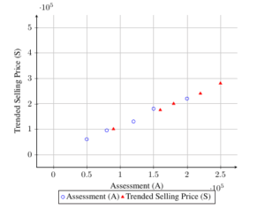
The linear regression traditionally used to test for vertical inequity, where \(Y = 0\) and \(\beta = 1/\gamma\). Unfortunately, model fails to meet classical linear regression assumptions because regressor \(S_i\) and error \((\epsilon_i + u_i)/\gamma\) correlate as per (2). Least squares estimations remain biased, persisting even with large samples, despite \(\gamma = 0\). Evaluating large-sample biases in least squares estimators necessitates assessing their probability limits. Empirical results from applying equation (1a) to a sample of 416 homes, are summarized in Table 1 and Figure 1, presenting statistics for \(A_i\), \(S_i\), and \(A_i/S_i\) data.
| Variable | Mean | Standard Error | A | S | A/S |
|---|---|---|---|---|---|
| A (Assessment) | 40000 | 8000.5 | 1.0 | 0.8507 | 0.0351 |
| S (Trended Selling Price) | 55000 | 20000.0 | 0.8507 | 1.0 | -0.6123 |
| A/S (Ratio) | 0.72727 | 0.15000 | 0.0351 | -0.6123 | 1.0 |

This section introduces refined regression techniques to accurately test vertical equity in property assessments. Each modification replaces traditional tests’ reliance on selling prices with assessments as regressors, mitigating false positives and detecting systematic deviations from equity. Our approach draws from general principles of estimator and forecast evaluation.
We advocate using the following regression model to test for uniformity: \[S_i = \alpha + \beta A_i + u_i\tag{4}\] If assessments are fair, Model (2) should accurately reflect the relationship between selling prices and assessments. Comparing Model (2) and our proposed Model (10), where \(\alpha = 0\) and \(\beta = \gamma\), aligns with assumptions of classical linear regression. Efficient assessments ensure that \(A_i\) and \(u_i\) are uncorrelated, and ordinary least squares provide unbiased estimators with minimal variance for parameters. Under the assumption of uniform assessments without vertical inequity, we anticipate the following properties for the least squares estimates: the intercept (\(\alpha\)) should not significantly differ from zero, and the slope (\(\beta\)) should approximate \(\gamma\), the ratio of average value to average assessment.
Detecting forms of inequity such as regressivity (\(\alpha < 0\)) involves yield Model. A test based on Model would identify such inequities by rejecting the hypothesis \(\alpha = 0\) in favor of \(\alpha \neq 0\) if supported by the data.
For the King County sample, the regression results for Model are as follows: \[S_i = \text{placeholder} + \text{placeholder} A_i \quad R^2 = \text{placeholder}\tag{5}\]
In the context of property assessment equity, assuming invariant variance of disturbances like \(u_i\), \(E_i\), or their sum \(q_i\) with respect to property value may not be reasonable. Typically, the variance of these errors increases proportionally with property value. This observation using residuals from the regression of \(S_i\) on \(A_i\), based on the King County sample.
While heteroscedasticity does not alter the core findings of earlier sections, it can impact tests relying on regression. Ordinary least squares in the presence of heteroscedasticity yields inefficient estimates and downwardly biased standard errors. Consequently, heteroscedastic errors may erroneously suggest significant departures from assessment uniformity even when the correct approach to regression bias is employed [11].
Various authors, have recognized this issue. Reinmuth suggests weighted least squares with transformed variables, albeit retaining bias problems. In our linear model, if errors \(q_i\) exhibit heteroscedasticity (\(V(q_i) = \sigma^2 A_i\)), a straightforward transformation by \(1/\sqrt{A_i}\) homogenizes the error variances. This approach is appropriate for testing linear bias amidst heteroscedastic errors.
A model where errors enter multiplicatively, effectively addressing heteroscedasticity. However, Cheng’s model retains the error associated with overlooking assessments as predictors of selling price, rendering his proposed test invalid. We advocate the following approach:
Assume selling prices for each property are randomly distributed around an unobserved value, \(S_i = V_i e^{u_i}\), with multiplicative errors \(e^{u_i}\) such that \(E(u_i) = 0\) and \(V(u_i) = \sigma^2_u\). Assessments (adjusted for a constant factor) serve as unbiased predictors of value, operationally reflected as selling price: \(V_i = \gamma A_i e^{e_i}\) or \(S_i = \gamma A_i e^{e_i} + \phi_i\), where assessment error \(e_i\) satisfies \(E(e_i) = 0\) and \(V(e_i) = \sigma^2_e\).
This model supports an effective test for assessment uniformity. The log transformation yields: \[\log S_i = \mu_i + \alpha \log A_i + q_i,\tag{6}\] where \(\mu_i = \log \gamma\) under the null hypothesis of uniform assessment. Ordinary least squares applied to regression can test this hypothesis.
For the King County sample, the log-transformed regression results are as follows: \[\log S_i = 0.8775 + 0.9720 \log A_i \quad R^2 = 0.6538\tag{7}\] The slope coefficient insignificantly differs from one, suggesting no evidence to reject the uniform assessment hypothesis. If anything, a coefficient less than one indicates slight progressivity (Table 2 and Figure 2).
| Category | Mean | Standard Deviation | Coefficient of variation | R-squared |
|---|---|---|---|---|
| Assessment Accuracy | $20,349 | $6,691.5 | 0.33 | 0.7727 |
| Trended Selling Price | $37,995 | $15,207.0 | 0.40 | 1.0 |
| Assessment/Selling Price Ratio | 0.56349 | 0.12942 | 0.23 | -0.5379 |
| Regression Results (Equation 12) | $2050.07 | $1527.93 | 0.37 | -0.713 |
| Residual Variance | 9.4338 x \(10^-6\) | |||
Cheng’s version gives: \[\log A_i = 2.8255 + 0.6727 \log S_i \quad R^2 = 0.6538\tag{8}\] According to standard interpretation, these results suggest significant regressivity, but bias invalidates this interpretation. The bias-corrected slope coefficient \(\alpha\) from this regression is \(\frac{\alpha}{1 – \sigma^2_u \log A_i} = 0.6727\).
Eliminating bias yields results consistent. The log-linear model effectively mitigates heteroscedasticity issues and generally outperforms previous linear models.
Even if a set of assessment data passes the tests for uniformity as recommended in previous sections, it does not necessarily imply that the assessments are optimal. Passing these tests simply indicates that significant improvement in assessments using only the current information is not feasible. Additional information could potentially lead to substantial enhancement in assessment accuracy. The criterion for assessing improvement is the reduction in residual variance in the regression of selling price on assessment and new information. If successful in reducing this variance, the new information can complement the existing assessment for constructing an improved version [12].
Borrowing terminology from efficient capital markets literature, we define an assessment procedure as weakly efficient if no significant improvement in assessments is possible using only the information contained within the assessments themselves. The tests discussed earlier provide assessments for weak efficiency. For instance, if the regression \(S_i = a + \beta A_i\) yields a significant intercept and a slope significantly different from unity, then using the old assessments as a basis allows us to construct new assessments using the relation \(A_{i,\text{new}} = a + \beta A_{i,\text{old}}\). When tested with the new assessments, the regression should ideally show a zero intercept and a slope of one.
Assessments are termed semi-strongly efficient if improvement in assessments, in terms of reducing residual variance, is not possible using objective property information currently available to the assessor’s office. Assessments are strongly efficient if improvement is not possible using any objective property information whatsoever.
We present a test for semi-strong efficiency using King County data. Our dataset includes one variable potentially enhancing assessments: adjusted grade, a subjective scale reflecting construction quality. The test involves adding this variable or variables to the regressors in the test equation. If adding new variables alongside the current assessment does not reduce residual variance, then the current assessment is semi-strongly efficient with respect to this new information. Conversely, if the new variable effectively reduces residual variance (analogous to a weak significance test using a Student t critical value of unity), we conclude that the current assessment can be improved using this data. The new variables, along with the old assessment, can then be used to generate an improved assessment.
Adding the adjusted grade variable \(Z_i\) to regression yields: \[\log S_i = 3.7548 + 0.5867 \log A_i + 0.14292 Z_i \quad R^2 = 0.6943\tag{9}\] The introduction of the new variable results in a reduction in residual variance, indicating that the assessment can be improved with the inclusion of adjusted grade in the dataset.
The procedure proposed to test for semi-strong efficiency can readily apply to variables currently available to the assessor’s office. Extending this to other unavailable data involves critical policy evaluation, weighing the increased cost of new data against the potential benefits of more accurate assessment and forecasting of selling prices (Table 3).
| Key Points | Details |
| Evaluation Context |
The paper discusses evaluating the quality of assessments as
forecasts or estimates for selling prices in real estate. |
| Efficiency Criteria |
Assessments are considered efficient if they cannot be improved using
only the assessment or the data on which it is based. |
| Correlation |
Efficient assessments have forecast errors uncorrelated with the
assessment itself but correlated with actual selling prices. |
| Traditional Tests |
Critique of traditional tests that erroneously concluded bias in
assessments due to correlations between assessment errors and actual selling prices. |
| New Methodologies |
Proposal of new tests to evaluate assessment efficiency and
potential for improvement using additional data. |
| Example Data |
Pilot sample dataset from King County, used to
illustrate concepts and methodologies. |
In many contexts, evaluating the quality of a forecast or estimate for a variable where the true value cannot be determined at the time of estimation is crucial. This challenge arises in various fields, such as finance, intertemporal consumption choice, and efficient fiscal policy. It is essential to distinguish between the estimate and the variable it predicts and to employ statistical models that accurately reflect their relationship.
Real estate assessments are forecasts or estimates of selling prices based on an incomplete set of property information. Evaluating assessments parallels the assessment of other forecasts or estimates. An assessment is considered efficient if, given the available data, it cannot be improved using only the assessment itself or the data upon which it relies. Consequently, the forecast error from an efficient estimate will be uncorrelated with the assessment but correlated with the actual selling price. This outcome is a consequence of the efficiency of the estimate and does not imply bias in the forecast or estimate. Moreover, it is valuable to investigate whether an assessment can be enhanced as a predictor of selling price using additional information not initially included in the assessment.
Traditional tests for assessing assessment quality have often conflated these issues, leading investigators to mistakenly conclude bias in assessments due to correlations between assessment errors and actual selling prices. This paper scrutinizes the shortcomings of traditional tests and proposes new methodologies for evaluating efficiency and the potential for improving assessments. These concepts are demonstrated using a pilot sample dataset from properties in King County. Traditional tests applied to this dataset reveal.