
The housing market has its own unique characteristics, belonging to rigid demand, with no low value and profitability, and no small added value. At the present stage, China’s economy is developing rapidly, urbanization is accelerating, and the demand for housing by urban residents is particularly high. Therefore, many investors and developers, driven by interests, invest in technology and large amounts of money to carry out housing development, so as to obtain higher profits[1-4]. In fact, while there are high profits in the housing market, there are also great uncertainties, high risks and many kinds of risks, which are mainly manifested in macroeconomic risks, policy risks, market supply and demand risks, capital risks and construction quality risks, etc. Therefore, reasonable risk management is crucial for the healthy development of the housing market[5-8].
As an important economic field, risk management of housing market is crucial for its healthy development. And the key of housing market risk management lies in the market research and analysis, diversified investment portfolio, flexible financial policy, strict quality control and effective risk monitoring and early warning mechanism[9-11], so as to effectively cope with the risk of the housing market and ensure the stability and healthy development of the market. Only by effectively managing the housing market and reducing its risks can we provide investors with safer and more reliable investment opportunities and create a better and safer investment environment for housing market participants[12-15].
Literature[16] aimed to discuss the risk management of selected private and non-profit affordable housing providers, through interviews to understand their risk assessment strategies in managing their programs, the study showed that informal risk management processes are also part of normal business processes in compliance with industry standards and that the level of acceptance of risk varies from one housing provider to another. Literature[17] reviewed information on macroprudential measures to reduce risk in the housing market and collated that the available information does not have relevant assessments of causality against different measures. Instead, a combination of household-level based data and policy reforms can provide insights into the effects of these measures. Literature[18] describes an integrated risk management framework that includes measuring credit portfolio risk, implementing stress tests, and so on, for capturing housing market cycles. A methodology based on the FAVAR approach extracts information from a set of housing market variables and applies a combination of estimated systematic factors to housing market risk management. Experiments confirm that the proposed methodology is well suited for analyzing slow-moving capital form risk. Literature[19] examines the explanation of the holding puzzle by focusing on housing and other uninsured risks. By using the French Household Wealth Survey as an example, it is found that the share of financial wealth invested in equities depends mainly on information costs, trading, and housing risk exposure, which are required to be acquired by controlling for endogenous home ownership status. Literature[20] takes the housing market in Jinan, China, over several years as the object of study, and uses a combination of quantitative and qualitative risk assessment methods to develop an analysis of the risk assessment and management of the housing market in Jinan, and proposes management measures that have practical effects in view of the risk assessment results. Literature[21] aims to explore the meaning of the developmental state of institutional capital inflow in private housing, adopting a generalized Hamiltonian Monte Carlo Bayesian approach, and finds that the inflow of capital signals a reduction in housing price uncertainty and vertical risk, emphasizing the significant impact of institutional capital on the housing market. Literature[22] revisited the issue of international diversification of housing securities and attempted to solve the problem of estimation errors in the input parameters by using alternative techniques, which showed a high improvement in the stability of the computed portfolio allocations with respect to other approaches. Literature[23]takes China’s housing loan market as an object and discusses the growth of the housing market and the role of banks in the housing market, using the government’s policies related to the regulation of home mortgages as a guide, and analyzes the risks in the housing loan market, the causes and the policies for mitigating the risks. Literature[24] provides an extensive risk assessment framework for portfolio management of real estate foundations in India, which is obtained by using hierarchical analysis based on numerous factors and standard risk prioritization. The results of the study show that risk prioritization for real estate portfolio management is most critical at the investment stage of the risk, while the most important thing to focus on is at the detection stage.
Compared with traditional risk management methods, the innovation is that this paper refines to the whole process risk management of housing market, including risk identification, evaluation and control. A cloud model is introduced to evaluate the risk of the housing market, realizing the conversion process from expert scoring to risk evaluation. Based on the developer’s perspective, a more complete and targeted housing market risk indicator system is constructed. The combination of information entropy-ANP method is used to calculate the weights of the indicators. Finally, the market risk of GJ housing project is comprehensively evaluated and the effectiveness of the evaluation method is tested. On this basis, risk control countermeasures are proposed.
It is common to define the uncertainty of loss as risk, which has the mathematical form[25]. Where denotes the risk, P denotes the probability of the risk occurring, and denotes the severity of the risk. So risk refers to a function of the degree of uncertainty (probability) about the consequences of the risk, and about the degree of uncertainty that gives rise to the risk. And the greater the probability and severity of the risk, the greater the risk that arises. And the existence of risk is not subject to human consciousness. Just because people anticipate a risk, they cannot go on to completely eliminate it in the course of their subsequent behavior.
Housing market risk refers to the uncertainty of loss that a real estate developer faces in the process of developing, constructing, and selling a residential project due to the uncertainty of the environment and conditions, as well as the influence of other human factors, which makes the actual outcome of the residential project deviate from the developer’s initial goal.
Variety
Due to the long development process of residential projects, the many links and specialties involved, as well as the participation of many different units, making the developer face more uncertainty.
Comprehensive
As the housing market is a complex and huge system, various influencing factors are intricate and interact with each other.
Ambiguity
Different risks have different probabilities of occurrence, and the probability of each risk occurring at different stages of development may also be different.
Large Losses
If the housing market risk occurs, most of it will have an adverse effect, and will cause different degrees of losses in terms of project schedule, quality and cost.
Risk management, is a dynamic control process that uses rational methods to maximize risk reduction under specific conditions. Risk management is mainly divided into three steps, risk identification, risk evaluation, risk control. Such a division can be well used to recognize, understand and manage risks with the idea of system theory, and can be well combined with the
characteristics of project management.
Risk Identification
Risk identification refers to finding out the potential risk factors in the process of project through appropriate methods. These risk factors are then analyzed to gain an in-depth understanding of their characteristics and the law of mutual influence to achieve the purpose of qualitative analysis. The housing market development cycle is long, the process is complex, and there are many influencing factors. So the identification work is heavy and complicated. Due to the defects of some theories, it is sometimes difficult to make qualitative description of some risk factors.
Risk Evaluation
On the basis of risk identification, further evaluation of potential risks, to understand their characteristics and development patterns, to determine how these risk factors affect the consequences of the project and its degree of impact. It is now more popular to evaluate these risk factors quantitatively through a series of methods, and the quantitative results must be reflected in recognized indicators. According to the quantitative results combined with the qualitative analysis of the evaluation stage, the risks are categorized and predicted to provide a basis for risk control.
Risk control
Risk control is a dynamic process of using effective methods to minimize the role of risk in the actual work process. According to the degree of impact of various risks derived from risk evaluation, risk factors are categorized into levels. For high-ranking risks, focused control is carried out to optimize the allocation of work resources.
The scientificity of the influence relationship between risk evaluation indicators and the weighting usually depends on the subjective judgment of experts, so this study carries out a scientific and objective design of the process that requires expert judgment when applying the information entropy-ANP method in order to improve the validity of the data. Through the information entropy model, it can clearly reflect whether the system is orderly or not, and also the size of the degree of order In order to ensure the professionalism of the experts, this time, 20 experts were invited, including professionals related to the field of investment and construction, and so on. The first step in constructing the network structure of ANP is to establish a control layer to clarify the goal of the problem, i.e., the risk evaluation of the housing market. Next, the network layer is established to clarify the risk indicators, and each risk element consists of multiple secondary risk indicators. Based on the information entropy method for the extraction of key risk factors, the portrayal of the causal relationship between risk factors, and the description of internal and external feedback and interaction relationships, the judgment relationship between risk factors is obtained. Experts’ opinions are asked and adjusted for conflicting judgment relationships, and consistency tests are conducted for each set of judgment matrices.
Expert evaluation to analyze and judge the relationship between indicators
First of all, the expert scoring, scoring guidelines for the five-point system, for the impact of factor \(a_{i}\) on \(a_{j}\) to develop the following scoring rules, 0 (no impact), 1 (small impact), 2 (- general impact) and 3 (large impact), 4 (very large impact). The diagonal in the matrix is the ratio to itself, so the values are all 0.
Constructing the direct impact matrix
The experts then do a two-by-two comparison based on the degree of influence between the risk factors, initially generating a \(n\times n\)st order matrix \(Z\), where \(a_{ij}\) represents the influence of element \(i\) on element \(j\). For the questionnaires of different experts take the mean value of each value \(\overline{a}\), and then determine the final \(a_{ij}\) according to the following formula, so as to build the direct influence matrix \(Z\): \[\label{GrindEQ__1_} Z\mathop{\scriptscriptstyle\leftharpoondown}\limits^{\displaystyle\rightharpoonup} =\left[\begin{array}{ccccc} {a_{11} } & {…} & {a_{1j} } & {…} & {a_{1n} } \\ {\vdots } & {} & {\vdots } & {} & {\vdots } \\ {a_{i1} } & {…} & {a_{ij} } & {…} & {a_{in} } \\ {\vdots } & {} & {\vdots } & {} & {\vdots } \\ {a_{n1} } & {…} & {a_{nj} } & {…} & {a_{nn} } \end{array}\right] , \tag{1}\] \[\label{GrindEQ__2_} \alpha _{ij} =\left\{\begin{array}{l} {0,0\le \bar{\alpha }<0.5} \\ {1,0.5\le \bar{\alpha }<1.5} \\ {2,1.5\le \bar{\alpha }<2.5} \\ {3,2.5\le \bar{\alpha }<3} \\ {4,,3.5\le \bar{\alpha }<4} \end{array}\right. . \tag{2}\]
Normalization of the direct influence matrix \(X\)
Sum the rows of the matrix, select the maximum value of the matrix \(Z\) for normalization, and finally obtain the normative impact matrix, denoted as \(X\): \[\label{GrindEQ__3_} X=S*Z , \tag{3}\] \[\label{GrindEQ__4_} S=\min \left\{\frac{1}{{\mathop{\max }\limits_{1\le i\le n}} \sum _{j=1}^{n}\alpha _{ij} } ,\frac{1}{{\mathop{\max }\limits_{1\le j\le n}} \sum _{i=1}^{n}\alpha _{ij} } \right\},i,j=1,2,…n . \tag{4}\]
Calculation of the integrated impact matrix \(T\) \[\label{GrindEQ__5_} T=X(1-X)^{-1} . \tag{5}\]
Calculation of the degree of influence of each element and the degree of influence, center degree and cause degree
The degree of influence is the sum of the values of each row in Matrix \(T\), which is used to indicate the degree of combined influence of the elements of each row on all other elements, denoted as \(D_{i}\), then: \[\label{GrindEQ__6_} D_{i} =\sum _{j=1}^{n}x_{ij} ,(i=1,2,3,…n) . \tag{6}\]
The degree of being influenced is the sum of the values of each column in matrix \(T\), which is used to indicate the degree of combined influence of each column element on all other elements, denoted as \(C_{i}\), then: \[\label{GrindEQ__7_} C_{i} =\sum _{j=1}^{n}x_{ij} ,(i=1,2,3,…n) . \tag{7}\]
The degree of centrality is used to indicate the position of the factor in the evaluation system and the degree of its influence, and the centrality of element \(i\) is obtained by adding its influence and influenced degrees, which is denoted as \(M_{i}\), then: \[\label{GrindEQ__8_} M_{i} =C_{i} +D_{i} . \tag{8}\]
The degree of cause of the original element \(i\) is obtained by subtracting the degree of influence and the degree of being influenced, denoted as \(R_{i}\), then: \[\label{GrindEQ__9_} R_{i} =D_{i} -C_{i} . \tag{9}\]
A cause factor with a value of \(>0\) on the cause scale indicates a high degree of influence on other factors, while a cause factor with a value of \(<0\) on the cause scale is called a result factor and indicates the degree of influence by other factors.
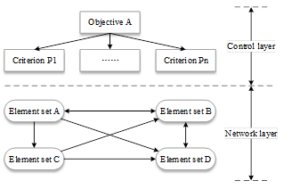
Establishment of ANP structure
The typical structure of ANP is shown in Figure 1, which includes a control layer and a network layer, where the guidelines in the control layer do not affect each other, and each set of elements or elements in the network layer affect each other[26].
Establishment of comparison judgment matrix for element groups and between elements
According to the ANP network structure diagram, it is possible to compare the importance of the elements within each group under the same elemental criterion to form the elemental comparison matrix, and at the same time, the comparison of the importance of each elemental group among themselves under the same elemental group criterion will also form the elemental group comparison matrix. In this paper, numerical values 1 9 are used to quantitatively analyze the importance of each factor as shown in Table 1, where each value represents a different meaning. Such an analysis method can assess the relative importance of each factor more scientifically and provide strong support for project decision-making.
| Degree of importance | Corresponding interpretation |
| 1 | \(y_i \) is as important as \(y_j \) |
| 3 | \(y_i \)is slightly more important than \(y_j \) |
| 5 | \(y_i \) is comparison important than \(y_j \) |
| 7 | \(y_i \) is significantly more important than \(y_j \) |
| 9 | \(y_i \) is more important than \(y_j \) |
| 2, 4, 6, 8 | Between the above assessment scale |
Consistency test of the matrix
In the construction of the judgment matrix, due to the need for expert scoring, there is a certain degree of subjectivity, in order to avoid contradictions between the elements, it is necessary to test whether the judgment matrix has consistency, the specific test method is to calculate the consistency ratio (CR), in which CR=CI/RI. CI indicates the consistency index, RI indicates the stochastic consistency index, when CR\(\mathrm{<}\)0.1, the judgment matrix has consistency, otherwise it does not have consistency. If the judgment matrix is inconsistent, it needs to be adjusted until it meets the consistency test standard. This ensures the accuracy and reliability of the judgment matrix.
Calculate supermatrix \(W\)
Let the column vectors in matrix \(W_{ij}\) correspond to the degree of influence of \(C_{j}\) on \(C_{i}\) in the control layer, respectively, then \(W\) is: \[\label{GrindEQ__10_} W=\left[\begin{array}{cccc} {W_{11} } & {W_{12} } & {\cdots } & {W_{1N} } \\ {W_{21} } & {W_{22} } & {\cdots } & {W_{2N} } \\ {\vdots } & {\vdots } & {} & {\vdots } \\ {W_{N1} } & {W_{N2} } & {\cdots } & {W_{NN} } \end{array}\right] . \tag{10}\]
Compute the weighted supermatrix \(\bar{W}\). \[\label{GrindEQ__11_} \bar{W}=(\bar{W}_{ij} ) , \tag{11}\] \[\label{GrindEQ__12_} \bar{W}_{ij} =u_{ij} \times W_{ij} , \tag{12}\] where \(i=1,2,…N;j=1,2,…N\).
Calculate the limit supermatrix \(\bar{W}^{\infty }\): \[\label{GrindEQ__13_} \bar{W}^{\infty } ={\mathop{\lim }\limits_{t\to \infty }} \bar{W}^{t} . \tag{13}\] From the information entropy model to derive the correlation degree of each risk indicator, ANP to derive the weight of each indicator, the combination of the two, the use of formula (10) to find out the comprehensive weight of the risk evaluation indicators, the comprehensive weight directly reflects the weight and degree of influence of each risk indicator in the system.
Calculate the risk priority ranking and determine the weights. \[\label{GrindEQ__14_} Z=W+T\times W=(1+T)\times W , \tag{14}\] where, \(Z\) is the hybrid weight, \(W\) is the weight of the indicator, \(T\) is the combined impact matrix of the indicator, and \(I\) is the unit matrix.
The cloud model can better describe the ambiguity and randomness and can reflect the intrinsic connection between the two, which can be applied to data processing to improve the precision of the evaluation results[27]. The housing market risk evaluation indexes established in this paper are qualitative indexes, which need to be quantified by expert scoring before risk evaluation. The cloud model can effectively deal with the conversion of qualitative and quantitative, and can effectively avoid the influence of subjective factors on the evaluation results, and the evaluation results are intuitive and easy to understand. Therefore, this paper introduces cloud modeling for housing market risk evaluation.
For real estate risk evaluation generally adopts five-level risk evaluation system, so this paper defines the housing market risk evaluation results as five levels, constituting For real estate risk evaluation generally adopts five-level risk evaluation system, so this paper defines the housing market risk evaluation results as five levels, constituting a set of rubrics as \(V=\{ v_{1} ,v_{2} ,v_{3} ,v_{4} ,v_{5} \}\)=\(\mathrm{\{}\)low risk, lower risk, general risk, higher risk, high risk\(\mathrm{\}}\), and each rubric level for bilateral constraints. Bilateral ranges \(V_{\max }\) and \(V_{\min }\) represent the maximum and minimum boundaries of the range of values of the rubrics, respectively, and the symmetric cloud model can be used to describe the rubrics with bilateral constraints, and the three numerical features are calculated by the formula: \[\label{GrindEQ__15_} \left\{\begin{array}{l} {E_{x} =\frac{(V_{max} +V_{min} )}{2} } \\ {E_{n} =\frac{(V_{max} -V_{min} )}{6} } \\ {H_{e} =k} \end{array}\right. , \tag{15}\] where \(k\) is a constant, can be adjusted in accordance with the degree of uncertainty of the rubric, generally take the value between 0.001 \(\mathrm{\sim}\) 0.1. In this paper, the golden section ratio method is used to partition the set of rubrics, and the closer to the center of the domain [0, 1], the smaller the values of evaluation levels \(E_{n}\) and \(H_{e}\). Taking the center point of the thesis domain 0.5 as the intermediate evaluation level (general risk), it has an expected value of \(Ex_{3} =0.3\) and a superentropy value of \(He_{3} =0.002\). According to the golden sectioning ratio, the multiplier of the cloud model parameter between adjacent levels of the rubrics is 0.645, and according to Equation (15), the cloud model parameter of each evaluation level is calculated as:
Expected value: \[\label{GrindEQ__16_} \left\{\begin{array}{c} {Ex_{1} =0} \\ {Ex_{2} =Ex_{3} -\frac{(1-0.645)(V_{max} +V_{min} )}{2} =0.311} \\ {Ex_{3} =0.3} \\ {Ex_{4} =Ex_{3} +\frac{(1-0.645)(V_{max} +V_{min} )}{2} =0.697} \\ {Ex_{5} =1} \end{array}\right. . \tag{16}\]
Entropy value: \[\label{GrindEQ__17_} \left\{\begin{array}{c} {En_{1} =\frac{0.645\times (V_{max} -V_{min} )}{7} =0.113} \\ {En_{2} =\frac{(1-0.645)\times (V_{max} -V_{min} )}{7} =0.065} \\ {En_{3} =\frac{0.645\times (1-0.645)\times (V_{max} -V_{min} )}{7} =0.038} \\ {En_{4} =\frac{(1-0.645)\times (V_{max} -V_{min} )}{7} =0.061} \\ {En_{5} =\frac{0.645\times (V_{max} -V_{min} )}{7} =0.103} \end{array}\right. . \tag{17}\]
Hyperentropy: \[\label{GrindEQ__18_} \left\{\begin{array}{l} {He_{1} =\frac{He_{2} }{0.645} =0.0137} \\ {He_{2} =\frac{He_{3} }{0.645} =0.0075} \\ {He_{3} =0.002} \\ {He_{4} =\frac{He_{3} }{0.645} =0.0075} \\ {He_{5} =\frac{He_{4} }{0.645} =0.0137} \end{array}\right. . \tag{18}\] As a result, the housing market risk comment set can be obtained, and its cloud model parameters are shown in Table 2. According to the data in Table 2, the forward cloud generator calculation using MATLAB software can be used to draw a cloud map of the comment set.
| Lv. | Evaluation criteria | Expected value (E\(_x\)) | Entropy (E\(_n\)) | Super entropy (H\(_e\)) |
| \(v_1 \) | Low risk | 0.0000 | 0.1130 | 0.0137 |
| \(v_2 \) | Relatively low risk | 0.3110 | 0.0650 | 0.0075 |
| \(v_3 \) | General risk | 0.3000 | 0.0380 | 0.0020 |
| \(v_4 \) | Relatively high risk | 0.6970 | 0.0610 | 0.0075 |
| \(v_5 \) | High risk | 1.0000 | 0.1030 | 0.0137 |
Expert survey scoring
This paper adopts the expert scoring method to determine the evaluation value of housing market risk evaluation factors. First, experts are made aware of the evaluation level, and then experts are invited to score each second-level indicator in the light of the specific conditions of the project, and the highest and lowest scores are given for the same indicator when scoring, i.e., bilateral constraint scoring is used.
Calculate the cloud number eigenvalues of the secondary indicators
According to the scoring results of the experts on the secondary indicators, the steps for calculating the numerical eigenvalues of the cloud model are introduced by taking a single risk indicator \(i\) as an example. There are \(n\) experts involved in scoring, and their highest and lowest scores for the same risk indicator \(i\) are \(x_{\max }\) and \(x_{\min }\), respectively. Using the inverse cloud generator, we can calculate the maximum and minimum cloud numerical eigenvalues of the risk indicator, and then calculate the cloud numerical eigenvalues:
First calculate the mean value: \[\label{GrindEQ__19_} \bar{X}_{max} =\frac{1}{n} \sum _{j=1}^{n}x_{\max i} . \tag{19}\]
The sample variance is then calculated: \[\label{GrindEQ__20_} S_{\max } {}^{2} =\frac{1}{n-1} \sum _{j=1}^{n}(x_{\max i} -\bar{X}_{\max } )^{2} . \tag{20}\]
Then, the maximum cloud digital eigenvalue is: \[\label{GrindEQ__21_} \left\{\begin{array}{l} {Ex_{\max } =\bar{X}_{\max } } \\ {En_{\max } =\sqrt{\frac{n}{2} } \frac{1}{n} \sum _{j=1}^{n}|x_{\max i} -\bar{X}_{\max } | } \\ {He_{\max } =\sqrt{\frac{|s_{\max }^{2} -En_{\max }^{2} |}{20} } } \end{array}\right. . \tag{21}\]
Similarly, the minimum cloud numeric eigenvalue \((Ex_{\min } ,En_{\min } ,He_{\min } )\) can be calculated, which in turn calculates the cloud numeric eigenvalue of a single risk indicator: \[\label{GrindEQ__22_} \left\{\begin{array}{l} {Ex=\frac{Ex_{max} En_{max} +Ex_{min} En_{min} }{En_{max} +En_{min} } } \\ {En=En_{max} +En_{min} } \\ {He=\frac{He_{max} En_{max} +He_{min} En_{min} }{En_{max} +En_{min} } } \end{array}\right. . \tag{22}\]
Similarly, the cloud digital eigenvalues of other secondary risk indicators are calculated. Through the above calculation, the cloud digital eigenvalues of the second-level risk evaluation indicators can be obtained.
Calculate the cloud digital eigenvalues of the first-level indicators
In this paper, there are 7 first-level risk evaluation indicators, and according to the cloud digital eigenvalues of the second-level indicators, the cloud digital eigenvalues of each first-level indicator can be calculated: \[ \begin{array}{c} {Ex=\frac{Ex_{1} Q_{1} +Ex_{2} Q_{2} +\cdots +Ex_{m} Q_{m} }{Q_{1} +Q_{2} +\cdots +Q_{m} } } \\ {En=\frac{Q_{1} {}^{2} }{Q_{1} {}^{2} +Q_{2} {}^{2} +\cdots +Q_{m} {}^{2} } En_{1} \cdots +\frac{Q_{m} {}^{2} }{Q_{1} {}^{2} +Q_{2} {}^{2} +\cdots +Q_{m} {}^{2} } En_{m} } \\ {He=\frac{Q_{1} {}^{2} +Q_{2} {}^{2} +\cdots +Q_{m} {}^{2} }{He_{1} } +\cdots +\frac{Q_{m} {}^{2} }{Q_{1} {}^{2} +Q_{2} {}^{2} +\cdots +Q_{m} {}^{2} } He_{m} } ,\end{array} \tag{23}\] where Q\({}_{i}\)\({}_{\ }\)is the comprehensive weight of each secondary indicator, \((Ex_{i} ,En_{i} ,He_{i} )\) is the cloud digital eigenvalue of each secondary indicator, and m is the number of evaluation indicators.
Establish the cloud model for comprehensive risk evaluation
By substituting the integrated weight \(Q_{i}\) and cloud number eigenvalue \((Ex_{i} ,En_{i} ,He_{i} )\) of each level indicator into Eq. (23), the cloud number eigenvalue of the comprehensive risk evaluation can be obtained, and then the forward cloud generator calculation can be carried out with the following steps:
Generate \(En{\rm {'} }\) with \(En\) as expectation and \(He\) as standard deviation.
Calculate the normal random number \(x\) by taking \(Ex\) as the expected value and \(En{\rm {'} }\) as the standard deviation, \(x\) which is a cloud drop for the qualitative concept.
Calculate the degree of certainty, \(y=exp\left[-\frac{(x-E_{x} )^{2} }{2E_{n}^{{'} } 2} \right]\).
Repeat steps 1\(\mathrm{\sim}\)3 until N cloud drops are generated.
In this paper, we utilize MATLAB software to calculate the forward cloud generator and draw a cloud diagram for comprehensive evaluation of housing market risk.
Combined with relevant research, as well as the experts’ description of the housing market risk, the finalized list of risk factors to realize the construction of the housing market risk evaluation index system is shown in Table 3. The risk evaluation system constructed in this paper consists of three levels: target layer, guideline layer and indicator layer respectively. Firstly, the housing market risk is taken as the target layer A, which is also the overall evaluation goal. Secondly, seven risk sources, including market (C1), technology (C2), society (C3), economy (C4), policy (C5), operation and management (C6), and natural environment (C7), are taken as indicators in the guideline layer, which is also used as the first-level indicators. Finally, the second-level indicators are the risk factors identified under each risk source, totaling 23 risk factors, which also serve as evaluation indicators for the indicator layer.
| Target layer | Criterion layer | Index level |
|
Housing market risk
(A) |
Market risk (C1) | Market supply and demand risk (C11) |
| Raw material supply risk (C12) | ||
| Price risk (C13) | ||
| Technical risk (C2) | Special requirements of design (C21) | |
| Technological innovation risk (C22) | ||
| Cost control risk (C23) | ||
| Construction quality risk (C24) | ||
| The progress risk of the period (C25) | ||
| Social risk (C3) | Urban planning (C31) | |
| Regional development level (C32) | ||
| Ethnic and religious practices (C33) | ||
| Economic risk (C4) | Financing risk (C41) | |
| Inflation risk (C42) | ||
| Changes in national economic conditions (C43) | ||
| Policy risk (C5) | Industry policy risk (C51) | |
| Land policy risk (C52) | ||
| Financial policy risks (C53) | ||
| Tax policy risk (C54) | ||
| Operation and management risk (C6) | Marketing risk (C61) | |
| Financial management risk (C62) | ||
| Personnel management risk (C63) | ||
| Natural environmental risk (C7) | Natural disaster (C71) | |
| Climatic conditions (C72) |
The GJ Housing Market project is located on the outskirts of an urban area in a third-tier city in the south. The project as a whole is oriented to the southeast, with fan-shaped rows, no interference between buildings, and abundant green landscape resources in the district. The external transportation conditions of the project are excellent, with the district government, urban forest park, sports park, as well as secondary and elementary school educational facilities to the north of the project, and access to the outskirts of the city and the vicinity of the highway to the south. Although the municipal park is rich in landscape resources, the project is in the outermost part of the city, and its peripheral living facilities are not yet perfect, and its project features co-development by branded real estate and enjoyment of branded real estate property services.
Residential project indicators as shown in Table 4, the residential project planning a total land area of nearly 165,000 square meters, a total construction area of nearly 456,000 square meters, the product mix of 36 sets of duplex villas, 10 30-35-story high-rise, 16 12-20-story high-rise, as well as a small portion of the street commercial composition.
| Indicators | Data |
| Occupied land area | 16,5000 m2 |
| Floor area | 45,6000 m2 |
| Plot ratio | 2.5 |
| Greening rate | 30% |
| Total cycle | 2400 |
| Building density | 0.2152 |
| Standard | Deluxe room |
| Vehicle space | 3205 |
The land plot of the project (replaced by the GJ project) was acquired by Company B through government auction, and the total transaction price was as high as 2.1 billion yuan, equivalent to a floor price of 12,727 yuan per square meter. With a total construction area of more than 450,000 square meters, the project is a large-scale development project in the local market environment.
The details of each risk evaluation index of the established housing market are designed to form a questionnaire, and it is issued to 20 experts for scoring the degree of importance, which come from universities, governmental agencies, real estate companies, construction units, and the experts score each risk evaluation index in the questionnaire according to their own accumulated experience using the Saaty 1-9 scale method as a way to Determine the value of each element in the judgment matrix. After the experts scored the raw data and processed the weighted geometric mean, the judgment matrix was formed, and then the weights of each evaluation index and the results of consistency test were obtained. The calculation results of the indicators of the judgment matrix A of the target and criterion levels are shown in Table 5. Among them, the weights of the seven first-level indicators (market (C1), technology (C2), society (C3), economy (C4), policy (C5), operation and management (C6), and natural environment (C7)) are 0.1818, 0.0945, 0.0527, 0.2306, 0.3452, 0.0607, and 0.0345, respectively. The consistency ratios (CR) are 0.0308 < 0.1, indicating that the break matrix is consistent.
| A | C1 | C2 | C3 | C4 | C5 | C6 | C7 |
| C1 | 1.0000 | 4.0000 | 2.0000 | 0.2500 | 0.1667 | 2.0000 | 5.0000 |
| C2 | 0.1667 | 1.0000 | 0.3333 | 0.1667 | 0.2000 | 4.0000 | 8.0000 |
| C3 | 0.2500 | 0.5000 | 1.0000 | 0.5000 | 0.2500 | 5.0000 | 6.0000 |
| C4 | 3.0000 | 4.0000 | 0.5000 | 1.0000 | 0.3333 | 0.1667 | 2.0000 |
| C5 | 0.2500 | 0.5000 | 4.0000 | 0.2000 | 1.0000 | 0.3333 | 3.0000 |
| C6 | 0.3333 | 0.2000 | 6.0000 | 3.0000 | 0.1250 | 1.0000 | 4.0000 |
| C7 | 0.2500 | 3.0000 | 0.3333 | 5.0000 | 2.0000 | 0.2500 | 1.0000 |
| Weight | 0.1818 | 0.0945 | 0.0527 | 0.2306 | 0.3452 | 0.0607 | 0.0345 |
| Consistency check | \(\lambda\))-max=7.3314, CI=0.0508, n=7, CR=0.03081 | ||||||
The calculation of indicator weights in the indicator layer is consistent with the solving steps of the criterion layer, and the comprehensive use of the information entropy-ANP method yields the results of the calculation of indicator weights as shown in Table 6. It can be seen that the consistency ratios (CR) among the second-level indicators are 0.0231, 0.0007, 0.0355, 0.0036, 0.1176, 0.0282, and 0.0000, respectively, which are all less than 0.1. It shows that the weights of the 23 calculated second-level indicators are reasonable, and they are recognized by the consistency of 20 experts.
| Criterion layer | Weight | Index level | Weight | CR |
| Market risk (C1) | 0.1818 | Market supply and demand risk (C11) | 0.5000 | 0.0231 |
| Raw material supply risk (C12) | 0.3000 | |||
| Price risk (C13) | 0.2000 | |||
| Technical risk (C2) | 0.0945 | Special requirements of design (C21) | 0.0482 | 0.0007 |
| Technological innovation risk (C22) | 0.1482 | |||
| Cost control risk (C23) | 0.2850 | |||
| Construction quality risk (C24) | 0.3715 | |||
| The progress risk of the period (C25) | 0.1471 | |||
| Social risk (C3) | 0.0527 | Urban planning (C31) | 0.5855 | 0.0355 |
| Regional development level (C32) | 0.2850 | |||
| Ethnic and religious practices (C33) | 0.1295 | |||
| Economic risk (C4) | 0.2306 | Financing risk (C41) | 0.6625 | 0.0036 |
| Inflation risk (C42) | 0.1356 | |||
| Changes in national economic conditions (C43) | 0.2019 | |||
| Policy risk (C5) | 0.3452 | Industry policy risk (C51) | 0.4450 | 0.1176 |
| Land policy risk (C52) | 0.1250 | |||
| Financial policy risks (C53) | 0.1372 | |||
| Tax policy risk (C54) | 0.2928 | |||
| Operation and management risk (C6) | 0.0607 | Marketing risk (C61) | 0.7155 | 0.0282 |
| Financial management risk (C62) | 0.1520 | |||
| Personnel management risk (C63) | 0.1325 | |||
| Natural environmental risk (C7) | 0.0345 | Natural disaster (C71) | 0.1665 | 0.0000 |
| Climatic conditions (C72) | 0.8335 |
In this paper, from the invitation of professionals, temporarily formed a specialized evaluation team (the team consists of 10 members, respectively, a company deputy manager, director, investment in the top, engineering department, cost department senior manager, GJ residential project manager and two college professors). Through the information that has been collected for each project, let the evaluation team personnel combined with the actual situation of the project, in accordance with the prescribed evaluation criteria to judge the indicators, get the GJ residential project various risk indicators scoring results as shown in Table 7. Which is listed as the evaluation team, the behavior of 23 risk evaluation indicators, the evaluation results for the 100-point system.
| Risk factor | Appraiser | |||||||||
| NO.1 | NO.2 | NO.3 | NO.4 | NO.5 | NO.6 | NO.7 | NO.8 | NO.9 | NO.10 | |
| C11 | 41 | 41 | 29 | 69 | 70 | 58 | 55 | 54 | 49 | 37 |
| C12 | 33 | 52 | 39 | 27 | 30 | 40 | 36 | 41 | 33 | 53 |
| C13 | 24 | 28 | 31 | 36 | 30 | 45 | 72 | 64 | 42 | 35 |
| C21 | 60 | 45 | 60 | 54 | 56 | 33 | 28 | 36 | 45 | 33 |
| C22 | 19 | 24 | 24 | 28 | 25 | 20 | 19 | 14 | 14 | 36 |
| C23 | 72 | 53 | 51 | 66 | 59 | 64 | 65 | 68 | 70 | 62 |
| C24 | 41 | 50 | 29 | 42 | 40 | 62 | 47 | 47 | 64 | 35 |
| C25 | 44 | 24 | 17 | 26 | 25 | 37 | 34 | 34 | 27 | 13 |
| C31 | 66 | 63 | 65 | 55 | 59 | 60 | 52 | 46 | 42 | 70 |
| C32 | 53 | 51 | 68 | 56 | 60 | 47 | 43 | 42 | 35 | 22 |
| C33 | 35 | 41 | 28 | 28 | 36 | 22 | 47 | 46 | 49 | 31 |
| C41 | 41 | 55 | 57 | 67 | 65 | 65 | 52 | 57 | 44 | 35 |
| C42 | 68 | 57 | 49 | 46 | 47 | 64 | 59 | 58 | 73 | 60 |
| C43 | 48 | 57 | 43 | 69 | 72 | 66 | 55 | 57 | 65 | 57 |
| C51 | 59 | 65 | 60 | 58 | 64 | 57 | 53 | 46 | 46 | 45 |
| C52 | 41 | 33 | 51 | 35 | 38 | 20 | 65 | 73 | 48 | 48 |
| C53 | 20 | 44 | 24 | 29 | 36 | 28 | 37 | 39 | 37 | 30 |
| C54 | 25 | 53 | 27 | 31 | 30 | 56 | 33 | 25 | 29 | 35 |
| C61 | 19 | 23 | 10 | 12 | 15 | 35 | 31 | 25 | 20 | 15 |
| C62 | 75 | 69 | 64 | 77 | 75 | 46 | 78 | 77 | 77 | 62 |
| C63 | 84 | 81 | 78 | 80 | 74 | 71 | 75 | 85 | 66 | 60 |
| C71 | 71 | 44 | 55 | 50 | 45 | 32 | 62 | 60 | 43 | 46 |
| C72 | 68 | 55 | 67 | 61 | 71 | 77 | 73 | 71 | 57 | 71 |
Based on the above data, the cloud model was used to calculate the cloud eigenvalues of the secondary risk indicators of the GJ housing market, and the specific results are shown in Table 8. The calculation found that the \(V_{min}\) and \(V_{max}\) of the expected values of the 23 risk factors are 18.284 and 79.6207, respectively, and the bilateral range indicates the maximum and minimum boundaries of the range of values of the rubric.
| Risk factor | Expected value \(E_x\)) | Entropy \(E_n\)) | Super entropy \(H_e\)) |
| C11 | 51.1912 | 10.5520 | 3.4511 |
| C12 | 44.2919 | 10.1242 | 2.5647 |
| C13 | 40.5312 | 12.4950 | 3.5065 |
| C21 | 43.9757 | 8.4111 | 2.5574 |
| C22 | 18.2844 | 2.3725 | 1.4918 |
| C23 | 66.8114 | 4.3604 | 2.1246 |
| C24 | 41.6298 | 11.3783 | 2.4230 |
| C25 | 29.6614 | 7.7738 | 2.4410 |
| C31 | 61.3148 | 8.3370 | 1.9995 |
| C32 | 43.6556 | 10.3712 | 5.5184 |
| C33 | 39.7239 | 7.7848 | 2.2790 |
| C41 | 56.6845 | 11.1056 | 1.9303 |
| C42 | 64.7458 | 7.8853 | 2.0155 |
| C43 | 57.0426 | 6.1197 | 2.9525 |
| C51 | 59.4161 | 8.8511 | 0.8257 |
| C52 | 47.3698 | 10.8151 | 7.2024 |
| C53 | 27.5382 | 7.7564 | 1.2685 |
| C54 | 34.7622 | 10.4547 | 1.2640 |
| C61 | 23.7620 | 9.8138 | 1.3790 |
| C62 | 73.0895 | 10.1915 | 4.8138 |
| C63 | 79.6207 | 8.9559 | 2.0062 |
| C71 | 49.0038 | 9.6320 | 3.1405 |
| C72 | 66.9298 | 7.1300 | 2.7694 |
| Risk factor | Expected value \(E_x\)) | Entropy \(E_n\)) | Super entropy \(H_e\)) |
| C1 | 43.6290 | 10.2370 | 2.9754 |
| C2 | 42.7214 | 8.3298 | 2.7123 |
| C3 | 39.4823 | 9.0008 | 2.6966 |
| C4 | 56.2266 | 9.4466 | 2.1870 |
| C5 | 42.5274 | 9.9521 | 2.5446 |
| C6 | 50.6632 | 10.8450 | 3.6339 |
| C7 | 43.4799 | 7.2861 | 2.6761 |
According to the revised comprehensive weight of risk indicators and the calculated eigenvalues of each secondary indicator cloud parameter, with the help of the cloud model established in the previous section of the comprehensive evaluation of risk, the characteristic parameters of each level of risk indicator cloud can be obtained, and the results of the calculation are shown in Table 9. Based on each level of risk indicator cloud, MATLAB software is used to assist in drawing its corresponding cloud map, and the drawing results are compared with the standard cloud map to visually determine the risk level of the risk type according to its relative position.
Market risk: The environmental risk cloud parameter is C1 (43.6290, 10.2370, 2.9754) and it is observed that the distribution of market risk in the GJ housing project is basically between lower and medium risk, with its cloud crossing between 65% and 75% certainty with the medium risk cloud and having a crossover of about 20% certainty with the lower risk cloud. From this, it can be concluded that the environmental risk in the GJ housing market is at a moderately low level.
Technological risk: The economic risk cloud parameter is C2 (42.7214, 8.3298, 2.7123), and the economic risk is mainly distributed between 20 and 50, focusing on about 38, and has a slightly higher crossover with the medium risk standard cloud map. From this, it can be concluded that the technical risk of the market is at a moderately low level.
Social Risk: The social risk cloud parameter is C3 (39.4823, 9.0008, 2.6966), which is mainly distributed between 30 and 60, focuses on about 45, and crosses more parts with lower risk. From this, it can be considered that the social risk of the market is at a lower level.
Economic Risk: The economic risk cloud parameter is C4 (56.2266, 9.4466, 2.1870), and the risk cloud map of GJ residential project is mainly distributed between 50-90, focusing on about 62, with more intersecting parts with the medium risk cloud map, and there are a larger portion of the cloud droplets dispersed within the cloud map of higher risk level. From this, it can be considered that the economic risk of the project is at a moderately high level.
Policy risk: The policy risk of the market is distributed between 30-50, focusing on about 35. The cloud droplets it produces wrap the medium risk cloud map and a smaller portion appears in the lower risk and higher risk cloud map. Therefore, the market policy risk can be considered as moderately low.
Management: Management risk cloud droplets are mainly distributed in the range of 20-75, focusing on 54, the cloud droplets are more dispersed, wrapped in the “general risk” cloud map, and the project management risk can be considered to be medium level.
Natural environment: The natural environment is clustered around 45, most of the cloud drops are distributed in the medium risk and low risk, and a few risk drops appear in the high risk cloud diagram. Combined with the weights of 7 level 1 indicators, using formula (23), the comprehensive risk distribution of the market of GJ residential project is between 31-54, focusing on 41. mainly medium risk, a small number of risk droplets appearing in the higher risk cloud map, the evaluation results are consistent with the actual.
According to the previous section combined with the qualitative analysis results of the evaluation stage, it can provide a basis for risk control. This paper proposes the following risk control strategies for the market risk of GJ residential project.
Risk avoidance: In the architectural design of commercial residential buildings, it is necessary to take into account the risks that may occur in a number of links, and to successfully avoid this and the corresponding work to carry out the trouble. Therefore, in the architectural design, in the design of the various stages such as the development of the task design book, the selection of construction materials and equipment and other aspects of the risk should be fully prepared for the design. Take corresponding risk avoidance measures, develop corresponding control points program, and through the control procedures to strengthen the process of control measures. At the same time, lessons should be learned from previous designs, and the relatively mature practices of advanced enterprises in the same industry should be utilized to enhance the corresponding technical capabilities.
Risk transfer: In the architectural design of residential projects, the risk should not be borne only by the design company, the design, construction, audit and final completion of the commercial housing between the participation of multiple units. In order to avoid the design company to bear too much risk, part of the risk should be transferred, by the multi-party subject to bear the risk factors of the whole stage. Risks are shared or transferred out through the signing of relevant contract terms. And before the start of the project, all parties should send representatives to participate in the project start-up meeting and feedback the basic situation. Before the architectural design institute starts the architectural design, the survey and design unit should first carry out an in-depth survey of the construction site, and bear the risk of whether the site construction conditions are available.
Risk Response: First of all, to communicate with the owner in the pre-design period to understand, in order to clarify the owner’s design needs, get the design intention and specific design requirements, to the overall design pointed out the general design direction, in order to facilitate the design process can be more smooth to get the final design goals. Then, refined to the design of commercial residential interior, this aspect requires coordination and cooperation between the various functional departments of the design institute to complete this part of the design, and the design of the interior of the building also needs to be coordinated with the construction part of the coordination together. For the internal communication and organizational coordination of commercial building design, the completion of the coordination process is indispensable, which should be established for the characteristics of this project project coordination procedures, and arrange for special staff responsible for the use of this part of the function, to ensure that the design of the internal and external to achieve timely communication and exchange, and standardization of communication methods and reporting systems.
Finally, for the project’s innovation, innovation is not only the design can also be the construction side of the innovation to optimize the overall structure and related components, which includes the relevant risks and hazards, including fire or earthquake and other disaster risk may cause substantial harm to the results of the above optimization and control. The main purpose of this process is to better realize the risk control, to reduce the possible impact of risk, and control.
This paper takes risk management, information entropy and cloud model as the theoretical basis, and carries out risk management on the housing project market from three steps of risk identification, evaluation and control, and takes GJ residential project as an example to study, which fills in the blank point of the current research on the risk management of real estate, and at the same time innovates in the establishment of the evaluation method. The research gets the following conclusions:
Based on relevant studies and expert surveys, this paper has sorted out that the risks of the housing market mainly originate from seven aspects: policy, economy, market, technology, society, operation and management, and natural environment, and finally constructed a risk evaluation index system containing 7 guideline-level indicators and 23 indicator-level indicators.
This paper chooses the cloud model evaluation method, which is less applied in the current field, to establish the market risk evaluation model, and combines the cloud model with the information entropy-AHP method to evaluate the risk of the housing market.
The following conclusions are drawn from the example of GJ housing: policy risk, market risk, and economic risk belong to “medium risk”, while business management and technology risk are between “low risk” and “medium risk”. Management and technology risks, while falling between “lower risk” and “medium risk”, are more inclined to medium risk. Social risks and natural environment risks are low risks. The overall risk evaluation of the housing project is medium risk, and the conclusion is in line with the actual situation, which verifies that the evaluation method is operable and feasible. Summarize. Through the three steps of risk identification, evaluation and control of the housing market, this paper has initially realized the risk management of the housing market. In the future, it can continue to select more scientific and reasonable management methods than this paper through in-depth research.