A Study of the Quantitative Impact of Different Credit Policies on Real Estate Price Volatility in the Housing Finance Market

I. Introduction

As a pillar industry of the economy, the real estate industry is not only the main carrier of wealth for ordinary families, but also the relative stability of real estate prices is related to the sound development of China’s national economy [1]. Real estate is both the real economy and a special form of virtual economy, real estate bubble development will continue to attract capital influx, resulting in the real economy financing environment of the “crowding out effect” [2,3]. As real estate prices continue to rise, forcing labor costs and investment costs to rise rapidly, indirectly increasing the cost burden of China’s real economy, reducing the ability of China’s industries to compete in the international market [4-6]. The rapid rise in real estate prices, the development of bubbles and bank credit associated with the risk of the questioning has aroused a high degree of social concern.

From the institutional level, the national real estate control policy is affected by “land finance”, excessive financial real estate and other reasons, there is the phenomenon of gaming between market players, local policies and national macro real estate control policy [7,8]. At the same time, real estate is also the most important investment direction of Chinese common family assets, the stability of real estate prices is related to the preservation and appreciation of the wealth of the Chinese common family, the sense of access and social stability, financial security [9,10]. In order to achieve the goal of stabilizing land prices, housing prices and expectations of the steady development of the real estate market, the establishment of a long-term mechanism has been the direction of the national macro-level real estate regulation and control constantly explored, the state has launched a series of loosening of the right to approve the construction of land, real estate enterprise financing, “three red lines” and other macro-control policies [11-14]. In order to maintain the stability of China’s real estate market prices, the study of bank credit on real estate prices, whether from the point of view of economic development, value preservation and appreciation of the wealth of residents and families, or from the point of view of financial security and social stability are of great practical significance.

Shen et al. [15] analyzed the changes in the capital structure of real estate listed companies during the credit expansion in China, and found that the before-and-after leverage and loan ratios of state-owned enterprises (SOEs) were elevated to a greater extent than those of non-SOEs, which caused the former to pay a higher land price than the latter, verifying the intrinsic mechanism by which the credit market exerts its influence on the real estate market. Liu [16] studied the impact of national credit policy changes on the real estate industry and put forward optimization suggestions on housing loan policies from the public standpoint, including the purchase of ownership housing, the improvement of housing conditions and the optimization of industrial structure. Kelly et al. [17] constructed a model of real estate prices related to the level of individual credit and the model showed that a 10% increase in credit received led to a 1.5% increase in the value of the property purchased by the borrower, which suggests that macro credit policy has an impact on low house prices and that the level at which it is set and the timing of its introduction are the key factors contributing to the extent of the impact. Greenwald et al. [18] developed a frictional rental market model to study the impact of credit-insensitive agents on house prices, and the results of the study showed that the rental market is highly frictional, explaining to some extent the phenomenon that a change in credit standards will elevate the house price-to-funding ratio. Robstad [19] explored the impact of monetary policy on real estate prices and household credit in Norway, monetary policy shocks have a strong impact on house prices and can be used to protect against financial instability, while the impact of monetary policy on household credit is weak, and monetary policy causes a decline in GDP and a change in inflation when mitigating easing household credit. Singh et al. [20] pointed out that asset prices in emerging markets are subject to shocks from credit and monetary policies, as demonstrated by the significant impact of bank credit on house price volatility. Bauer [21] assessed the factors affecting the prediction of real estate price revisions in terms of monetary policy expectations measured using an international term structure model with a time-varying risk premium, and real estate prices estimated using an asset pricing model, which showed that market expectations of high policy interest rates would increase the likelihood of house price revisions. Cuestas et al. [22] examined the interdependence between house prices and housing credit in Estonia and found that negative housing credit innovations would have a significant impact on house prices, implying that the central bank could mitigate house price volatility by increasing the capital buffer in times of boom to set the stage for credit policy in times of economic hardship.

The article proposes a quantitative analysis model combining the stock-flow model and the VAR model, which is applied to the quantitative analysis of real estate price fluctuations by different credit policies to provide a quantitative analysis basis for the optimization of different credit policies and the precise regulation of real estate prices in the housing finance market.

Since the housing market reform, the real estate industry has experienced a sustained and rapid development, which has played an important role in improving people’s housing demand and stimulating economic growth, and has gradually become a pillar industry of the national economy. This paper analyzes the symbiosis and transmission mechanism between credit policy and real estate prices based on the theory of supply and demand equilibrium price theory and real estate cycle fluctuation theory. Based on the stock-flow model of real estate prices, a PVAR model is established with the vector autoregression model to analyze the impact of credit policy on real estate price fluctuations. China’s real estate-related data from 1998 to 2023 are selected for empirical analysis, and the regional and price growth rate heterogeneity of different credit policies in the housing finance market is explored.

II. Theoretical foundations

Living and working in peace and contentment has been the pursuit of the people’s life since ancient times, and living in peace and contentment is the basic guarantee for work and life, so it can be seen that “living” has always been the most basic needs of the people. However, along with the rapid development of the real estate industry, real estate prices are rising faster and faster, the contradiction between supply and demand in the real estate market has become increasingly severe, the ordinary people are increasingly looking at the house sigh. Whether it is real estate developers, or the main body of the purchase of real estate in the development and purchase of real estate in the process are inseparable from the support of credit policy, credit policy in the real estate industry plays a pivotal role. Therefore, the study of credit policy and real estate prices between the impact of the relationship has important practical significance.

I. A. Relevant theoretical foundations

I. A. 1) Equilibrium price theory of supply and demand

In the case of a perfectly competitive market, the supply and demand for a commodity combine to form the equilibrium price of the commodity. At this point, the supply and demand of goods are equal, and the market reaches equilibrium, the specific state as shown in Figure 1. Price changes will bring changes to the supply and demand of commodities, resulting in oversupply or undersupply in the market, and changes in market supply and demand will affect the formation of equilibrium price and trading volume [23].

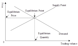
Factors affecting the movement of the equilibrium point of price supply and demand come from the price of the commodity itself, the level of consumer income, consumer preferences, the price of related commodities, population, and other demand-side factors. Influences on the supply side include the prices of factors of production, the government’s tax system, and the level of production technology and management. The development of the national economy and population, the overall national economic operations of the city, and the development of the residential industry. The residential industry can often contribute to the development of the national economy, and the sustained and stable operation of the national economy improves the living conditions of the residents, while raising their income levels and expanding their purchasing power, keeping developers and buyers expecting better from the residential market. Along with the increase in urban population, the demand for residential housing will also expand.

I. A. 2) Real estate cycle fluctuation theory

The real estate cycle cycle is generated by the poor coordination of supply and demand in the market. Whereas economic activity is cyclical in nature, the demand for space exhibits cyclical movements. The real estate cycle is divided into four processes: recovery, expansion, contraction, and recession.

1. Recovery phase. Early stage of recovery phase: due to the excess construction and negative growth rate of demand in the previous phase, the housing vacancy rate reaches its highest value at the lowest point of the cycle, and then enters the recovery phase. As real estate supply is still greater than demand, real estate prices and market rent levels are still low, but they begin to rise slowly from low levels, and real estate investment activity is low and almost non-existent during this period.

2. Expansion stage. Further macroeconomic expansion, accelerated economic growth and social return on investment steadily increased, prompting increased corporate earnings, consumer demand has grown rapidly, the real estate market entered a phase of prosperity, the volume of market transactions continued to grow significantly, the vacancy rate fell further.

3. Contraction phase. The majority of market participants still rely on market regulation to stabilize the economic growth trend, believing that the lowest point of the vacancy rate has already passed, and continue to build on the real estate market. However, the real estate market shows the market condition of price drop and volume contraction, due to the increased risk of real estate long investment, the scale of real estate investment is reduced, and a large number of speculators exit the market.

4. Recession stage. Accompanied by the overall tightening of the macro economy, the cleaning of the real estate bubble, surviving real estate development enterprises to quality, real estate prices began to stabilize. The state issued a series of policies to stimulate economic recovery, and subsequently demand began to increase.

I. B. Transmission mechanism of credit policy

I. B. 1) Symbiosis between credit policy and real estate prices

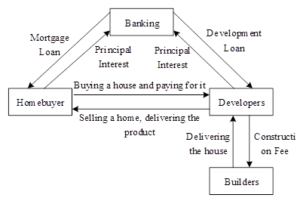
The real estate capital chain demonstrates the role played by credit policy in the various segments of the real estate market, the capital flows from the bank to home buyers and developers, and flows back to the bank in the circular process shown in Figure 2. At present, real estate financing is relatively single, the vast majority of the source of funds or bank loans. Developers apply for development loans from the bank, the capital flows from the bank to the developer, after the developer obtains the working capital, it can carry out the construction of premises, part of the capital is used for land turnover, part of the funds need to be paid to the real estate builder for the construction of the house, which is when the developer will be in the market for the sale of the period house or the existing house [24]. On the other hand, the demand for housing by applying to the bank for a mortgage loan to purchase a home, the funds flow from the bank to the buyer, the buyer with the funds loaned by the bank to pay to the developer to obtain real estate products, the developer with the sale of housing proceeds from the funds to pay the bank loan and interest. At this point, the real estate capital chain to complete a cycle. In the process of a complete cycle, bank credit plays an absolute supporting role, and the bank also obtains interest income from it, realizing a win-win situation for the real estate market and the bank.

I. B. 2) Credit policy affects real estate prices

Bank credit policy mainly in the form of development loans and housing mortgage loans into the real estate market, and formed the main component of real estate development funds, the size of which determines the scale of real estate investment and construction. According to the general market supply and demand theory, if the bank gives the real estate development loan scale increases, the real estate housing supply will increase, at this time if the housing demand remains unchanged, the price of housing will fall. However, the actual real estate prices have not decreased, the main reasons are as follows:

First, the limited land resources for building houses, coupled with the lag in the supply of real estate, resulting in the supply and demand in the real estate market can never be balanced, real estate supply exceeds demand for a long time, which in turn gives developers more power to decide on the price of housing. Secondly, due to the information asymmetry between supply and demand, developers have a more comprehensive grasp of the real situation of housing, so developers can determine the price of housing through the supply of real estate. Finally, because commercial banks provide real estate developers with sufficient development funds, consumers can not delay the purchase of housing and thus reduce personal housing loans into real estate development and construction, which further enhances the developer’s right to determine the price of housing, and therefore in the long term prices continue to rise.

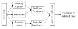
The way credit policy affects real estate prices is shown in Figure 3. First of all, by controlling the money supply to affect the size of credit, and then further affect the real estate market available funds, development loans and personal loans increased respectively caused by the increase in supply and demand for real estate, due to the lag in the supply of housing, resulting in the real estate market demand exceeds supply, and house prices rise further. Secondly, changes in the size of credit produce interest rate effects, bank credit expansion, loan interest rates are lower, investors and home buyers will be more inclined to buy real estate, real estate demand increases, and then housing prices continue to rise. Finally, people will be because of the expected future growth and decline in housing prices to decide whether to buy a home, when the credit crunch, people expect that future housing prices may decline, and thus begin to reduce the demand for real estate consumption. For investors, the expected return on their investment in real estate decreases, so the demand for both investment and consumption in the real estate market decreases.

III. Study design

Looking back on the development of the real estate market, the up and down fluctuation of housing prices not only brings obstacles to the stable development of the economy, but also raises the cost of living of the residents and reduces the residents’ sense of well-being, therefore, how to regulate housing prices within a reasonable range is an important issue related to the stable development of the country, the national well-being of the people. Government departments have been actively taking relevant policies and measures to regulate the real estate market, and in the measures to regulate the real estate market over the years, the control of credit policy has been regarded as the main measure. But from the credit measures taken by the government on the real estate market control effect, credit policy is not always effective and timely control of the real estate market, housing prices are still in the state of up and down again and again, failed to remain within a reasonable range.

III. A. Real estate price research model

III. A. 1) Stock-flow modeling

This paper analyzes the impact of credit policy on real estate price volatility by drawing on the “stock-flow” model proposed by existing related studies. The model assumes that there are two main actors in society, i.e., real estate and the banks that provide financial support to real estate developers, and does not take into account other environmental factors such as investors’ willingness to invest, market distribution, and the economic cycle for the time being.

Assuming that current demand in the real estate market \(D_{t}\) is inversely related to market house prices \(P_{t}\) and positively related to credit facilities \(L_{t}\) provided by banks, and that credit facilities \(L_{t}\) available to home buyers from banks banks are in turn inversely related to interest rates \(r_{t}\) and positively related to incomes \(Y_{t}\) and market prices \(P_{t}\), this can be expressed by the following equation: \[\label{GrindEQ__1_} D_{t} =\frac{L\left(Y_{t} ,r_{i} ,P_{t} \right)}{P_{t} } . \tag{1}\]

By analyzing the above assumptions, we can get \(L_{Y} >0\), \(L_{p} >0\), and \(Lr<0\).

We use \(\alpha\) to denote the depreciation of the stock of houses, \(K_{t}\) to denote the current stock, and \(I_{t}\) to denote the current flow, and stock \(K_{t}\) is the value of the houses in the current period net of depreciation plus the flow added in the previous period, which can be expressed by the equation: \[\label{GrindEQ__2_} K_{t} =(1-\alpha )K_{t-1} +I_{t-1} . \tag{2}\]

Assuming that the output of real estate, i.e., the new flow, depends on the size of the amount of bank financing, and that the amount of credit extended by the bank is directly proportional to the income, the price of the property, and inversely proportional to the market rate of interest, and that we denote the amount of financing funds obtained by the real estate from the bank’s borrowing sector by \(B\), with \(\beta\) as the coefficient, the equation can be expressed as follows: \[\label{GrindEQ__3_} I_{t-1} =\beta B\left(Y_{t-1,} ,r_{t-1} ,P_{t-1} \right) . \tag{3}\]

From the above analysis, \(Br_{y} >0\), \(B_{p} >0\), \(Br<0\).

When market equilibrium is reached, i.e., market demand equals market supply, then \(D_{t} =K_{t}\).

We substitute the above equation to obtain: \[\label{GrindEQ__4_} K_{t} =\frac{L\left(Y_{t} ,r_{t} ,P_{t} \right)}{P_{t} } . \tag{4}\] \[\label{GrindEQ__5_} K_{t} =(1-\alpha )K_{t-1} +\beta B\left(Y_{t-1,} r_{t-1} ,P_{t-1} \right) . \tag{5}\]

From the above model, we can see that bank credit and real estate prices have a two-way positive relationship, the supply of funds from bank credit is affected by interest rates, incomes and house prices, once the supply increases, it will have a positive impact on the demand for real estate, and the increase in demand in turn leads to an increase in the equilibrium price of real estate. At the same time, due to the small supply elasticity of real estate, so the increase in credit funds will lead to a direct increase in real estate prices in the short term. And real estate prices if rising at the same time will also affect the amount of bank credit, the rise in house prices increased market supply, for the growth of demand for bank credit, at the same time, between the collateral asset quality is in a benign upward trend, the bank also has to increase the willingness to put.

III. A. 2) Vector autoregressive model

Vector Autoregressive (VAR) models are able to better represent the dynamic associations of multiple variables with each other, thus compensating for the shortcomings of traditional econometrics in which only static relationships can be represented. The VAR model is suitable for analyzing the dynamic effects of stochastic perturbations on the system as well as predicting the time series system, which essentially tests the dynamic interactions between multiple variables, overcoming many of the problems brought about by the constraints of economic theories to which previous economics regression models are subjected, and at the same time avoiding the problem of missing variables [25]. Therefore, this paper proposes to analyze the relationship between different credit policies and real estate price volatility in the housing finance market using a VAR model.

The expression of VAR model is as follows: \[\label{GrindEQ__6_} Y_{t} =Z_{1} Y_{t-1} +Z_{2} Y_{t-2} +\ldots +Z_{n} Y_{t-n} +\varepsilon , \tag{6}\] where \(Y\) is the vector of \(K\)-dimensional endogenous variables, \(Z\) denotes the matrix of coefficients, \(n\) denotes the order in which the endogenous variables are lagged, \(t\) denotes the lag period, and \(\varepsilon\) is a constant term.

In general, constructing a VAR model needs to include the following six parts:

1. Unit root test to test whether the data applied to this paper are smooth to avoid pseudo-regression.

2. Determine the lag order of the VAR model, so as to construct the VAR model.

3. VAR model stability test, to verify whether the established VAR model is stable.

4. Granger test, to test the causal relationship between variables.

5. Impulse response analysis, to analyze the dynamic impact of mutual shocks between the variables.

6. Variance decomposition, to explore the extent to which each variable in the model contributes to the model.

III. B. Variable selection and model construction

IIII. B.1) Selection of research variables

This paper comprehensively compares and analyzes the direction and size of the impact of each variable on real estate prices, taking into account the optionality of the data, the main variables selected are real estate prices (PRICE), total real estate credit (TLOAN), real estate development loans (BLOAN), personal housing loans (MLOAN) and bank lending rates (BLR).

1. Real Estate Prices. Since monthly data on real estate prices are not published in the statistical database, monthly data on real estate prices can only be obtained by dividing the sales of commercial properties by the area of real estate commercial properties sold and using the resulting average sales price of commercial properties as an indicator of real estate prices.

2. Total real estate credit. Total real estate credit with real estate development loans and personal housing loans data can be summed up. According to the real estate asset pricing theory, real estate prices and expected returns into a positive relationship, if the expected return on real estate rises, the current real estate prices will be higher. As the expansion of real estate credit scale will increase investors’ expectations of the current and future upward economic development, the expected future value of real estate as an asset will rise, thus increasing the current real estate prices.

3. Real estate development loans are bank loans to real estate developers, mainly including commercial banks to real estate developers of domestic loans part. So real estate development loan data indicators are expressed in terms of real estate investment domestic loan data. Resident personal housing loans using personal mortgage loan data, personal mortgage loans are commercial banks to borrowers for the purchase of housing loans, accounting for the main part of personal housing loans.

4. Loan interest rates. In accordance with the theory of real estate asset pricing, real estate prices and the discount rate into an inverse relationship. A rise in the discount rate reduces the price of real estate. Since the discount rate includes the market interest rate component, from a theoretical point of view, the interest rate and real estate prices is also an inverse relationship. Considering the long repayment period of real estate loans, the bank loan interest rate adopts the “Medium and Long Term Loan Interest Rate above 5 Years” announced by the Central Bank to reflect the level of bank loan interest rate.

III. B. 2) Research modeling

Based on the real estate price “stock-flow” model and VAR model given in the previous section, this paper adopts the panel vector autoregression model (PVAR) to analyze the data on the basis of the panel data of real estate price fluctuations. Combined with the variables selected in the previous section, the PVAR model is constructed as follows: \[\label{GrindEQ__7_} \left\{\begin{array}{l} {PRICE_{t} =\alpha _{0} +\phi _{1} TLOAN_{t} +\phi _{2} TLOAN_{t-1} +\cdots +\phi _{p} TLOAN_{t-p} +\varepsilon _{t} } \\ {PRICE_{t} =\beta _{0} +\phi _{1} BLOAN_{t} +\phi _{2} BLOAN_{t-1} +\cdots +\phi _{p} BLOAN_{t-p} +\varepsilon _{t} } \\ {PRICE_{t} =\gamma _{0} +\phi _{1} MLOAN_{t} +\phi _{2} MLOAN_{t-1} +\cdots +\phi _{p} MLOAN_{t-p} +\varepsilon _{t} } \\ {PRICE_{t} =\delta _{0} +\phi _{1} BLR_{t} +\phi _{2} BLR_{t-1} +\cdots +\phi _{p} BLR_{t-p} +\varepsilon _{t} } \end{array}\right. \tag{7}\]

The PVAR model usually consists of three parts, firstly, a regression relationship between the variables is established, secondly, the impulse response function is analyzed to study the degree of influence of each factor on a certain factor as well as the number of persistence periods, and lastly, the variance decomposition analyzes the degree of influence of shocks with different information on the endogenous variables, thus further illustrating the degree of influence of each variable.

IV. Empirical studies

After the implementation of the housing system reform, the real estate industry entered a period of rapid development and quickly became a pillar industry of the national economy, playing a pivotal role in economic development. At the same time, the continuous loose monetary policy after the financial crisis has also made a large amount of money pouring into the real estate market, while the real economy is facing the serious challenge of “deconstruction to virtualization”. Commodity housing as a necessity of life, become the focus of people’s attention, the government is also taking corresponding measures to the real estate industry for a number of regulation. However, real estate prices continue to rise, and more than the general population’s purchasing power, the real estate market bubble tendency, the accumulation of risk, to a certain extent, to the whole society has caused adverse effects. For this reason, an in-depth study of the impact of different credit policies on real estate price fluctuations in the housing finance market will help to further optimize credit policies and promote the stable development of real estate prices.

IV. A. Data sources and variable statistics

IV. A. 1) Research data sources

This paper selects the annual panel data of 31 inter-provincial regions in China from 1998 to 2023 as the research sample, and the data are mainly obtained from the Wind database, the database of the National Bureau of Statistics (NBS), and the statistics database of the China Economy Network (CEN). Among them, the price of commercial housing, GDP per capita, disposable income of urban residents, construction cost of commercial housing, land price, real estate credit scale and total sales of commercial housing are all adjusted by CPI to get the real value, and the budgeted fiscal expenditure of local governments is adjusted by GDP deflator to get the real value. In order to eliminate the influence of data size on the empirical test, all variables are in the form of natural logarithms, except for the financial leverage ratio of the commercial housing development enterprises, the urbanization level and the CPI index.

IV. A. 2) Statistical characterization of variables

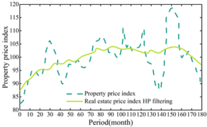
In this paper, the real estate market transaction price index data is selected as the real estate price data, and the dataset is obtained from the CEIC database, and this part focuses on the description of the statistical characteristics of this variable. Figure 4 shows the trajectory of the real estate price index and its HP filter over time. As can be seen from the figure, the real estate market price index has climbed since the implementation of the housing commercialization reform in 1998. From April 1999 to January 2008, the real estate market price has been increasing, while from 2008 to 2010, due to the impact of the world financial crisis, the real estate price has been decreasing. After the financial crisis, the real estate price index resumed its upward trend and reached its highest peak since 1999 around 2010. After that, the real estate price index decreased due to the government’s control of housing prices, and combined with the results of descriptive statistics, it can be seen that the real estate price index is close to the normal distribution but slightly right-skewed, while its HP filtered series is left-skewed and non-normally distributed series. In addition, in order to meet the needs of the research after this paper, this paper for the real estate price index series of the smoothness of the test, the ADF test results in the 1% significance level can not be rejected real estate trading price index of the original series of non-stationary series of the original hypothesis, and its first-order difference after the series in the 1% significance level to reject the unit root process of the original hypothesis. Therefore, it can be concluded that the real estate transaction price series is a unit root process, which implies that this series needs to be treated appropriately in the subsequent studies of this paper.

IV. B. Analysis of empirical results

IV. B. 1) Cointegration and Granger Tests

On the basis of carrying out the construction and analysis of the PVAR model, it is necessary to carry out the unit root test, the cointegration test and the Granger test for each variable in the model, which aims to emphasize the smoothness of the variables. Table 1 shows the results of the ADF test for each variable, where D() is the first-order difference.

For the non-stationary time series, some of the numerical characteristics of the series are changing with the change of time, that is to say, the non-stationary time series have their different stochastic laws at each point in time, and it is more difficult to grasp the overall stochasticity through the known information in the past. If we directly use the data of non-stationary time series for econometric analysis, it is easy to appear the phenomenon of pseudo-regression, so in the econometric regression before we first need to test the smoothness of the time series. After the ADF test on the original series, the results show that the P-value is greater than 0.05, which shows that the original series is not smooth, and there is a unit root that needs to be differentiated. After the first-order differencing of the original series, the series becomes smooth and all obey the first-order single integer, at this time the values of the variables in the smooth series can be regarded as randomly fluctuating according to a fixed level.

Table 1 Variables ADF test results

		Critical value			P	Stability
Variable	ADF	1%	5%	10%
LnPRICE	-3.215	-4.015	-3.463	-3.026	0.064	Uneven
LnTLOAN	1.073	-2.548	-1.958	-1.623	0.518	Uneven
LnBLOAN	1.284	-2.336	-1.849	-1.575	0.627	Uneven
LnMLOAN	1.527	-2.727	-1.902	-1.616	0.595	Uneven
LnBLR	-0.186	-3.485	-2.881	-2.578	0.939	Uneven
D(LnPRICE)	-3.299	-2.589	-1.946	-1.624	0.002	Stability
D(LnTLOAN)	-2.731	-2.583	-1.945	-1.625	0.001	Stability
D(LnBLOAN)	-2.582	-2.581	-1.946	-1.624	0.000	Stability
D(LnMLOAN)	-2.624	-2.585	-1.945	-1.624	0.005	Stability
D(LnBLR)	-9.215	-2.586	-1.943	-1.625	0.003	Stability

The purpose of the cointegration test is to determine whether a linear combination of a set of non-stationary series has a stable equilibrium relationship. When the series are non-stationary, there will be pseudo-regression phenomenon, so it is necessary to carry out differential processing, but this will cause the total amount of data to be reduced, so we have to carry out the cointegration test. In this paper, we use Johansen cointegration test method to carry out cointegration test for each variable, and the results of cointegration test are shown in Table 2. Based on the results of the cointegration test can be found, the trace statistic and the maximum eigenvalue test results are the same and there is at most one cointegration relationship between the two, because both in the At most 1 original hypothesis under the conditions of the P-value is greater than 0.05, accept the original hypothesis. So it can be considered that there is a long-term stable equilibrium relationship between the variables in the model.

Table 2 The results of the Cointegral test of each variable

Original hypothesis	Eigenvalue	Trace statistics	5% Critical value	P	Result
None	0.476	90.275	29.827	0.000	Reject
At most 1	0.081	12.818	15.496	0.124	Accept
At most 2	0.001	0.062	3.854	0.815	Accept
Original hypothesis	Eigenvalue	Trace statistics	5% Critical value	P	Result
None	0.476	78.669	20.163	0.001	Reject
At most 1	0.081	12.574	14.625	0.086	Accept
At most 2	0.001	0.062	3.854	0.815	Accept

The cointegration test is to determine whether there is a stable equilibrium relationship between the variables, while the Granger causality test is to determine whether the explanatory variables and the explained variables are causally related. The results of Granger test for each variable in this paper are shown in Table 3. As can be seen from the table, at the 5% level of significance, there is a bidirectional Granger causality between total real estate loans and real estate prices, and mutual Granger causality between bank lending rates and real estate prices.

Table 3 Granger test results of each variable

Original hypothesis	F statistics	Prob	Result
TLOAN is not PRICE’s granger reason	12.516	0.000	TLOAN is PRICE’s granger reason
BLOAN is not PRICE’s granger reason	5.948	0.001	BLOAN is PRICE’s granger reason
MLOAN is not PRICE’s granger reason	3.271	0.000	MLOAN is PRICE’s granger reason
BLR is not PRICE’s granger reason	2.995	0.003	BLR is PRICE’s granger reason
PRICE is not TLOAN’s granger reason	5.247	0.025	PRICE is TLOAN’s granger reason
PRICE is not BLOAN’s granger reason	3.482	0.017	PRICE is BLOAN’s granger reason
PRICE is not MLOAN’s granger reason	2.951	0.044	PRICE is MLOAN’s granger reason
PRICE is not BLR’s granger reason	3.006	0.029	PRICE is BLR’s granger reason
TLOAN is not BLOAN’s granger reason	2.151	0.028	TLOAN is BLOAN’s granger reason
TLOAN is not MLOAN’s granger reason	2.685	0.021	TLOAN is MLOAN’s granger reason
TLOAN is not BLR’s granger reason	3.047	0.009	TLOAN is BLR’s granger reason
BLOAN is not MLOAN’s granger reason	2.514	0.034	BLOAN is MLOAN’s granger reason
BLOAN is not BLR’s granger reason	2.446	0.017	BLOAN is BLR’s granger reason
MLOAN is not BLR’s granger reason	3.698	0.005	MLOAN is BLR’s granger reason

IV. B. 2) Impulse response analysis

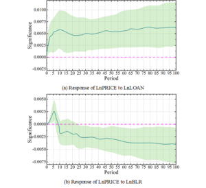
Since the PVAR model is not a purely theoretical model, it is possible to analyze the dynamic impact of an error term on the whole system, i.e. The impulse response, without any a priori constraints on the variables, or when the PVAR model receives a shock. In this paper, in order to verify the way credit policy affects real estate price volatility and to further determine the changes in the national economy that come with it, impulse response analysis has been carried out on the three variables PRICE, LOAN, and BLR, respectively. Figure 5 shows the results of the impulse response analysis, in which Figures 5(a)\(\mathrm{\sim}\)(b) show the response results when real estate prices are impacted by credit policy and when bank lending rates are impacted by real estate prices, respectively.

It is clear from Figure 5(a) that the response of real estate price volatility is inverted L-shaped. The level of real estate price volatility responds quickly after a shock of one standard deviation of credit policy is given (i.e., when there is an expansion in credit policy), showing a rapid increase. This response peaks at 0.00611 in period 10, meaning that a 1 percentage point expansion in the size of credit policy will increase real estate prices by 0.00611 percentage points. This rapid response from the perspective of real estate developers, because when the bank credit expansion, not only will put a large amount of money into the market, so that developers can expand the scale of financing to further expand investment, will also be accompanied by the bank on the market to relax the conditions of the credit business audit, so that the original can not be financed through the bank to get the opportunity to finance the enterprise, thus expanding the demand side of the credit market. From the perspective of home buyers, the expansion of bank credit scale, will greatly release the signal that housing prices are about to rise, increasing the public’s psychological expectations of the real estate market demand increases, thus contributing to the rise in housing prices. After reaching the peak, the increase in house prices appeared a short retracement, in the 100 period, the impact of bank credit policy on house prices tends to stabilize at 0.00625 percentage points. On the one hand, this is due to the fact that the market will gradually become rational after experiencing volatility, and on the other hand, it is due to the fact that the growth of the supply side and the demand side of real estate is gradually balanced.

As can be seen in Figure 5(b), credit interest rate has a positive impact on real estate prices in the short term, but the effect is very short, about 6-7 periods, then instantly becomes negative, and has been in a negative state since then. In the long run credit interest rates on real estate prices is a negative impact, the effect of the role of the effect gradually increased, and then stabilized, maintained at a stable value (-0.00375). That is, as the credit rate increases, real estate prices will decrease, that is, the increase in the credit rate will inhibit the increase in real estate prices, the decrease in the credit rate will contribute to the increase in real estate prices. Through the impulse response results can also be seen if you want to reduce real estate prices in the short term, increase the credit rate approach is not feasible, if you want to stabilize real estate prices in the long term does not rise, increase the credit rate approach is more reliable approach, but also to achieve the effect of the credit policy is more desirable approach.

IV. B. 3) Analysis of variance decomposition

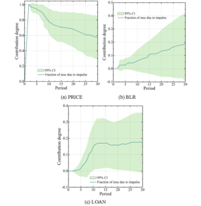
The variance decomposition is used to examine how much of the fluctuation of real estate prices is influenced by its own factors and how much is influenced by changes in credit policy and credit interest rates, i.e., it is possible to analyze the degree of contribution of credit policy (LOAN) and credit interest rates (BLR) to the fluctuation of the changes in real estate prices (PRICE) and to determine the degree of importance of the two explanatory variables. Figure 6 shows the results of the variance decomposition, where Figures 6(a)\(\mathrm{\sim}\)(c) show the degree of influence of real estate price, credit interest rate, and credit policy on real estate price, respectively.

Based on the results of the variance decomposition can be concluded that the real estate price in the early stage is mainly affected by their own factors, and the contribution can be up to 100%, the consumer’s expectation of real estate prices largely determines the change of real estate prices in the later stage, and with the passage of time this contribution gradually decreases, and finally stabilizes at about 58.98%. If the market believes that real estate prices will rise, it will cause many consumers to buy, leading to an increase in demand for housing and causing real estate prices to rise. If the market is bearish on real estate prices and believes that real estate prices will fall, then consumers postponing consumption will lead to a decrease in the demand for housing and a fall in real estate prices. Credit policy and interest rates on real estate prices have a lag period, in the short term credit policy on real estate prices compared to interest rates is in a dominant position, in the early part of the sustained and rapid rise, and after reaching the peak of the gradual stabilization of its contribution to real estate price fluctuations in the 19.87% or so. Credit interest rates have a smaller impact on real estate prices in the short term, but as time goes by it is getting bigger and bigger and keeps on rising, and finally the contribution of credit interest rates to the impact of real estate prices is around 17.04%. In conclusion, there is a significant positive impact of different credit policies on real estate price volatility in the housing finance market, with credit interest rates having a smaller degree of impact on real estate prices in the short term and a more pronounced long-term effect.

IV. C. Robustness tests and heterogeneity

IV. C. 1) Robustness tests

In order to verify the robustness of the results of the regression analysis of the PVAR model, this paper introduces the model constructed by cross-multiplying terms to calibrate the robustness of the conclusions of the PVAR model. The LOAN is decomposed into three dimensions, TLOAN, BLOAN and MLOAN, and the cross-multiplication term with BLR is used to construct the robustness model. Table 4 shows the robustness test results based on the cross-multiplying terms, where models (1) to (3) are the robustness test results of TLOAN*BLR, BLOAN*BLR, and MLOAN*BLR, and *** denotes that it is significant at the 1% level, and the robustness error is shown in parentheses.

In the regression results of the cross-multiplier term, the coefficients of TLOAN*BLR, BLOAN*BLR, and MLOAN*BLR on real estate prices are 0.0235, 0.0371, and 0.0214, respectively, all of which show significant positive impacts on real estate prices at the 1% level. With the expansion of credit policy, individual housing loans, real estate enterprise development loans, and bank loan interest show a stronger force on real estate price fluctuations, and all pass the robustness test at the 1% level. Based on the estimation results of the cross term coefficients in the table, the impact of credit policy on real estate price volatility is confirmed again, which is consistent with the findings of the PVAR model. Therefore, the paper concludes that the foregoing empirical findings are relatively robust.

Table 4 Stability test results based on cross-term

Variable	Model \eqref{GrindEQ__1_}	Model \eqref{GrindEQ__2_}	Model \eqref{GrindEQ__3_}
TLOAN*BLR	0.0235***(2.815)	–	–
BLOAN*BLR	–	0.0371***(2.938)	–
MLOAN*BLR	–	–	0.0214***(2.867)
(Cons_)	0.0924***(4.124)	0.145***(4.162)	0.139***(3.186)
AR (2)	0.746	0.515	0.569
Sargan	0.523	0.508	0.517
F statistic	8.947	9.032	9.125
R\(^2\)	0.815	0.816	0.814

IV. C. 2) Heterogeneity analysis

1. Heterogeneity results based on geographical stratification

   In order to further analyze the impact of different credit policies on real estate price volatility in the housing finance market, this paper divides China into three regions, namely, east, west and central, based on the traditional geographic stratification method given by the National Bureau of Statistics. And the fixed effect model (FE) and random effect model (RE) are constructed to empirically study the panel data of the three regions, and after the modified Hausmann test, the fixed effect model should be chosen for all three regions. Table 5 shows the results of the heterogeneity test for different regions, where *,**,*** denote significant at the 10%, 5%, and 1% levels, respectively, and standard errors are in parentheses.

   According to the empirical results show that in the economically developed eastern region, different credit policies in the housing finance market have a significant positive impact on real estate prices, and credit policy is an important reason for boosting real estate prices in the eastern region. While the central and western regions credit policy for real estate prices is not significant. From the empirical results of decomposition variables, residents’ income and the level of real estate investment, development and construction are the reasons for the impact of real estate prices in the central and western regions, and the impact of credit policy on real estate prices varies in different regions on the basis of traditional geographic stratification.

   Table 5 Heterogeneity test results in different regions

   Variable	Eastern region		Central region		Western region
   	FE	RE	FE	RE	FE	RE
   LnLOAN	0.249*** (0.121)	0.237*** (0.116)	0.048 (0.127)	0.059 (0.135)	0.138 (0.142)	0.121 (0.147)
   LnTLOAN	0.124** (0.041)	0.132*** (0.037)	0.029** (0.035)	0.006*** (0.038)	0.039** (0.034)	0.042* (0.025)
   LnBLOAN	0.042* (0.035)	0.015* (0.029)	0.007* (0.041)	0.002** (0.035)	0.025* (0.018)	0.009** (0.015)
   LnMLOAN	0.132*** (0.165)	0.137*** (0.177)	0.128*** (0.135)	0.157*** (0.168)	0.167*** (0.074)	0.158*** (0.061)
   LnBLR	-0.135** (0.072)	-0.176*** (0.068)	-0.075** (0.024)	-0.063* (0.034)	-0.047* (0.028)	-0.184** (0.025)
   CONS	0.268 (1.167)	-0.107 (1.186)	-0.215 (0.758)	-0.008 (0.835)	1.406** (0.535)	0.954** (0.481)
   HAUSMAN	Prob>chi2=0.089		Prob>chi2=0.001		Prob>chi2=0.000

2. Heterogeneity results based on price growth rate stratification

   Based on the above empirical study on the impact of credit policy on real estate prices, it can be seen that the role of credit policy in promoting real estate prices and the impact of different regions there are differences in the need for further consideration based on differences in the real estate market for heterogeneity analysis. Using the average annual growth rate of real estate prices as the basis for stratification, divided into fast-growing prices, medium-growing prices and slow-growing prices in the region. The panel data of the three regions stratified according to the new stratification method are empirically investigated using fixed-effects model and random-effects model respectively, while after the modified Hausmann test, the random-effects model is selected for fast-growing and slow-growing regions, and the fixed-effects model is selected for medium-growing regions. Table 6 shows the heterogeneity results based on price growth rate stratification.

According to the empirical results show that in the area of rapid growth in real estate prices, credit policy has a significant positive impact on real estate prices, which has a significant positive impact at the 1% level (t=0.283,p\(\mathrm{<}\)0.01). To the area of medium growth in real estate prices, credit policy still has a positive impact on real estate prices (t=0.161,p\(\mathrm{<}\)0.05), but compared to the fast-growth areas, the impact is weaker, and the significance is also weakened. And to the slow growth of real estate prices in the region, the direction of the impact of credit policy on real estate prices remains unchanged, but the impact is not significant (t=0.101,P\(\mathrm{>}\)0.1). It can be seen that the faster the growth rate of real estate prices in the region, the housing finance market in the different credit policy for the region’s real estate prices to boost the role of the greater.

Table 6 Heterogeneity results based on price growth stratification

Variable	Eastern region		Central region		Western region
	FE	RE	FE	RE	FE	RE
LnLOAN	0.283*** (0.154)	0.246*** (0.132)	0.135 (0.106)	0.161** (0.127)	0.101 (0.137)	0.105 (0.151)
LnTLOAN	0.133** (0.064)	0.131*** (0.052)	0.042** (0.085)	0.018*** (0.042)	0.047** (0.026)	0.045* (0.021)
LnBLOAN	0.065* (0.042)	0.047* (0.035)	0.009* (0.023)	0.005** (0.016)	0.038* (0.021)	0.029** (0.018)
LnMLOAN	0.117*** (0.134)	0.128*** (0.169)	0.118*** (0.151)	0.121*** (0.154)	0.135*** (0.068)	0.124*** (0.059)
LnBLR	-0.124** (0.086)	-0.135*** (0.093)	-0.028** (0.046)	-0.022* (0.041)	-0.034* (0.076)	-0.072** (0.083)
CONS	0.215 (1.089)	-0.226 (1.081)	-0.206 (0.847)	-0.105 (0.726)	1.228** (0.814)	0.981** (0.752)
HAUSMAN	Prob>chi2=0.609		Prob>chi2=0.092		Prob>chi2=0.776

V. Conclusion

The article analyzes the impact of different credit policies on real estate price volatility in the housing finance market using a panel vector autoregressive model. There is a significant positive shock response of credit policy on real estate price volatility, when the size of credit policy is expanded by 1 percentage point, real estate price will increase by 0.00611 percentage points. And there is a short-term positive effect of credit interest rate on real estate prices, which turns into a negative effect after the medium and long term. Driven by different credit policies in the housing finance market, real estate price fluctuations are most pronounced in the eastern region, while no such effect exists in the central and western regions. In addition, the faster the growth rate of real estate prices, the greater the degree of influence of credit policy. Therefore, the stabilization of real estate prices need to be combined with the actual situation of different regions and economic development, the formulation of corresponding credit policy, in order to achieve the precise control of real estate prices.