A Study on Spatial Differentiation of Urban Land Prices Based on Geographically Weighted Regression Models

I. Introduction

Dynamically changing urban land price is the wind vane and indicator of land market operation, reflecting the operation of the land market, and to a certain extent, also reflects the development of urban socio-economic life [1,2].

Urban land price information is a synthesis of natural, economic, social and other attributes, and thus affected by many factors, which is mainly reflected in the spatial and temporal changes of land price. The factors that cause changes in urban land prices interact with each other and are constantly changing in response to changes in the nature of the city, socio-economic development, and changes in the needs of urban residents [3-5]. The traditional statistical methods used for land price assessment often neglect the impact of land price itself as an explanatory variable on the surrounding land price, resulting in the averaging of land price in the whole region, failing to reflect the heterogeneity of land price in the region, and it is generally difficult to get a more satisfactory result [6-9]. In contrast, the spatial variable coefficient regression model, i.e., geographically weighted regression (GWR), allows different spatial relationships to exist in different geographic spaces, which largely reveals the spatial dependence and spatial non-smoothness of geographic phenomena [10-12]. Thus, the method of GWR was introduced into the measurement of urban benchmark land value assessment model, which provided a new method for conducting spatial exploratory analysis of urban land value [13-15].

Mou et al. [16] examined the correlation between housing prices and land in different cities in mainland China using a geographically weighted regression model, which showed that there was a significant positive correlation between land prices and house prices, while the relationship between land supply and house prices was not significant. Chen et al. [17] empirically analyzed the spatial homogeneity and non-stationarity of residential land prices by identifying geographic information factors such as geographic location, transportation accessibility, etc. using a traditional regression model and a GIS-based spatial autocorrelation model. Dell’Anna et al. [18] combined the feature pricing approach with GIS to explore the economic value of urban green infrastructure, spatially characterizing the market for residential units by measuring distances between land elements and considering dependency effects between residential unit transactions. Lan et al. [19] showed that spatial inequality in public service amenities exacerbates competition in the housing market and directly contributes to spatial heterogeneity in housing prices, and thus utilized a hybrid geographically weighted regression model and a geoprobe model to explore the relationship between house prices and urban public service amenities. Nakamura et al. [20] constructed a land price function based on a geographically weighted regression model, and analyzed the results of the influence of related factors on land price, which showed that entrepreneurship, social vitality, and environmental quality were significantly positively correlated with the price of land, and that the price of land in large cities was more influenced by entrepreneurship and social vitality. Yang et al. [21] used geographically weighted regression analysis with land price monitoring data to study the effects of foreign population, gross domestic product (GDP), and investment in residential construction on the dynamics of residential prices, and found that GDP contributes to housing prices in the Los Angeles region.

This paper takes land economics and other theories as the entry point, innovatively combines spatial data analysis method, geostatistical method and geographically weighted regression model, breaks the inherent thinking limitations, quantifies the law of spatial differentiation of urban land prices, and realizes the visualization research of urban land prices. The study identifies the residential land sales within the built-up area of QZ urban area during 2013-2022 as the research sample point, and determines the use of ESDA model with land price profile line (variation function and Kriging spatial interpolation) to carry out the study of spatial heterogeneity of urban residential land price. We also analyzed the influencing factors of the spatial variability of urban residential land prices from three aspects, namely, location factors, neighborhood factors, and individual factors of the parcels, using linear regression model and geographically weighted regression (GWR) model.

II. Research methods and models for spatial differentiation of urban land prices

II. A. Exploratory spatial data analysis

Exploratory spatial data analysis (ESDA) is a spatial analysis method that takes spatial correlation measurement as the core, describes and reveals the spatial distribution of the research object, discovers singular observations, and analyzes their spatial connections, clusters, and other heterogeneities. The method emphasizes the discovery of distribution patterns of spatial data, focusing on the visual phenomena of spatial correlation and spatial heterogeneity of data. Through ESDA, the attributes of the data, the structure of the data and its spatial distribution, the global trends of the data, and the spatial autocorrelation of the data can be understood. Exploratory spatial data analysis enables users to have a deeper and more comprehensive understanding of the data, so that they can better utilize the data for the study of related issues [22].

II. A. 1) Analysis of space data structures

In the study, it is necessary to use the ArcGIS geostatistical analysis tool to perform Kriging interpolation on the urban land price sample point data, and the data is normally distributed is the premise of Kriging interpolation, so before that it is necessary to analyze the spatial data structure of the urban land price data, and measure the normal distribution of the data.

In exploratory spatial data analysis, QQ plots are usually used to compare the distribution of existing urban land price data with the standard normal distribution. In QQ plots, the standard normal distribution is a straight line, so the closer the urban land price data is to the straight line, the closer it is to obeying the normal distribution QQ plots can be of two kinds: normal QQ plots and regular QQ plots. Normal QQ plots are mainly used to assess whether univariate sample data with multiple values obey normal distribution, and regular QQ plots are used to assess the similarity of the distribution of two data sets. Therefore, the normal QQ plot is used to assess the normal distribution of urban land price data in this paper.

The horizontal coordinate of the normal QQ plot is the ordinal number and the vertical coordinate is the cumulative probability. If the distribution of urban land price data in the normal QQ plot is a straight line, it indicates that the price data obeys a normal distribution. If there are outliers, i.e., there are individual sample points that deviate too much from the straight line, they should be tested. If the data does not show a normal distribution in the normal QQ plot, the data should be transformed to follow a normal distribution before using the Kriging interpolation method, where the Log transformation is generally used.

II. A. 2) Trend analysis

Trend analysis observes the spatial trend of the data and produces a three-dimensional perspective view of the data. In the trend analysis map, the geographic coordinates of the urban land sample points are projected on the x, y plane, with the x-axis representing the direction of longitude, i.e., east-west, and the y-axis representing the direction of latitude, i.e., north-south, and the price of urban land is projected on the z-axis in a one-to-one correspondence with the urban sample points, i.e., the height of each vertical bar in the trend analysis map represents the price of urban land, and the position of each vertical bar represents the geographic coordinates of urban land. It is also possible to isolate directional trends by rotating the data. In a nutshell, the sample points of the study area are converted into a 3D perspective view with the value of the attribute to be studied as the height, and by rotating this 3D perspective view, the global trend of the sample data set can be analyzed from different viewpoints.

To observe trends that exist in a particular direction, a line of best fit can be made through the projected points. If the line is flat, it indicates that no trend exists. Trend analysis is a simple and intuitive way to understand the spatial distribution of things.

II. A. 3) Spatial autocorrelation analysis

Urban land prices have the bulge sign of clustering in space, so the use of spatial autocorrelation analysis can well explore the spatial differentiation characteristics of urban land prices [23].

1. Global spatial autocorrelation

   Moran index comes from the Pearson correlation coefficient in statistics, which is actually the standardized spatial autocovariance. It tests whether the neighboring areas in the whole study area are similar (spatial positive correlation), dissimilar (spatial negative correlation), or independent. The formula of Moran’s I is as follows: \[\label{GrindEQ__1_} Moran^{{'} } I=\frac{n\sum\limits_{i=1}^{n}\sum\limits_{j=1}^{n}w_{ij} (x_{i} -\bar{x})(x_{j} -\bar{x})}{\sum\limits_{i=1}^{n}\sum\limits_{j=1}^{n}w_{ij} (x_{i} -\bar{x})^{2} } =\frac{\sum\limits_{i=1}^{n}\sum\limits_{j=1}^{n}w_{ij} (x_{i} -\bar{x})(x_{j} -\bar{x})}{S^{2} \sum\limits_{i=1}^{n}\sum\limits_{j=1}^{n}w_{ij} } . \tag{1}\]

   The standardized statistic Z of Moran’s I is: \[\label{GrindEQ__2_} Z(I)=\frac{I-E(I)}{\sqrt{VAR(I)} } , \tag{2}\] where \(E(I)\) is its theoretical expectation and \(VAR(I)\) is its theoretical variance.

2. Local spatial autocorrelation

   Global spatial autocorrelation is a general description of the entire study area, which assumes that the space is homogeneous, but because of the uneven spatial distribution of geographic elements, the real space is often not homogeneous, there is spatial heterogeneity, and the influence of the same influencing factors varies in different spatial regions, therefore, it is necessary to use the local spatial autocorrelation statistic to analyze spatial autocorrelation, and the commonly used The commonly used statistics are localized Moran’s I or LISA, localized Geary’s C and Gi index.The LISA of region \(\; i\) is used to measure the degree of correlation between region \(\; i\) and its neighbors, defined as: \[\label{GrindEQ__3_} I_{i} =\frac{(x_{i} -\bar{x})}{S^{2} } \sum _{j\ne i}w_{ij} (x_{j} -\bar{x}) . \tag{3}\]

At \(I_{i} >0\), it indicates positive spatial autocorrelation, where values with the same attribute cluster together, i.e., high values cluster with high values and low values cluster with low values, and at \(I_{i} <0\), it indicates negative spatial autocorrelation, where values with dissimilar attributes cluster together, i.e., a high value is surrounded by a low value (high and a low), or a low value is surrounded by a high value (low and a high).

The standardized statistic \(Z\) for LISA is: \[\label{GrindEQ__4_} Z(I_{i} )=\frac{I_{i} -E(I_{i} )}{\sqrt{VAR(I_{i} )} } , \tag{4}\] where \(E(I_{i} )\) denotes its theoretical expectation and \(VAR(I_{i} )\) denotes its theoretical variance.

II. A. 4) Spatial heterogeneity

The non-uniform or non-random distribution of spatial elements leads to spatial heterogeneity. Spatial heterogeneity, or spatial non-smoothness, means that things and phenomena in each spatial locus are characterized by characteristics that distinguish them from those in other loci.

Things and phenomena are spatially heterogeneous because the various things and phenomena themselves lack a smooth structure in space, and the spatial units themselves are not homogeneous, with great differences in area, shape, etc. The existence of spatial heterogeneity implies that not only the overall or total spatial pattern should be discovered, but also the local differences in spatial patterns should be recognized and the spatial difference characteristics should be revealed. According to the existing valuation theories and experiences, the influence of the same influencing factors varies in different locations, i.e., the relationship between land price and each influencing factor is not constant and varies according to the location.

II. B. Steps in geostatistical analysis

Geostatistics is a method of unbiased valuation of regionalized variables at future sampling points using the structural nature of the raw data and the semivariance function. Geostatistical analysis is generally divided into the following 3 steps:

1. Preliminary analysis of the raw data to calculate the sample capacity, sample mean, and sample variance, and to produce a histogram of the frequency distribution. This process is also known as exploratory analysis of data.

2. Calculate the value of the variance function and fit the variance function curve.

3. Apply the kriging method for spatial interpolation.

II. B. 1) Variational functions

Geostatistics is primarily used to detect the structure of spatial variation in spatial phenomena, as well as to estimate and model the values of variables. Regardless of the field of application, the core of geostatistical analysis is to determine the pattern of the study object with respect to spatial location based on sample points, and to use this to derive the value of the unknown point, which is also known as the variability function. The pattern of the variation function is shown in Figure 1.

\(Z(x)\) variation function (denoted by \(r(h)\)) in that direction, where \(h\) is an arbitrary spatial distance and \(N(h)\) is the number of pairs of sample points. For an observed series of data \(Z(x_{i} ),i=1,2,\cdots ,n\), the value of the sample variance function \(r(h)\) can be calculated using the following equation: \[\label{GrindEQ__5_} r(h)=\frac{1}{2N(h)} \sum _{i=1}^{N(h)}\left[\begin{array}{c} {Z(x_{i} )-Z(x_{i} +h)} \end{array}\right]^{2} . \tag{5}\]

When the corresponding variance function values are calculated for the samples in their spatial distribution area along a certain direction or all directions, the variance function values corresponding to their individual \(h\) values are labeled in the right-angled coordinate system with the horizontal coordinates as the spatial distances \(h\) and the vertical coordinates as the values of the semi-variance function, and the variance function pattern graph is formed.

In practice, the theoretical variance function model is unknown and often has to be estimated from valid spatial sampling data, a series of semivariance values can be obtained for a variety of different \(h\) values, and the distribution of the variance of the sample point pairs can be fitted with a function.

Currently, models of variance function curves in geostatistics include spherical, Gaussian, exponential, and linear models. The commonly used spherical model is: \[\label{GrindEQ__6_} r(h)=c_{o} +(c-c_{o} )\left(\frac{3h}{2a} -\frac{1}{2} \left(\frac{h}{a} \right)^{3} \right) , \tag{6}\] where \(c_{o}\) is the nugget value, which indicates the discontinuous variation in the regionalized variable at a scale smaller than the sampling scale, as determined by the attributes of the regionalized variable or the measurement error. \(c\) is the abutment value, which is the largest variation in the system or system property, and \(a\) is the range of variation, which is the distance between intervals when \(r(h)\) the abutment value is reached, and it indicates that after \(h\ge a\) the spatial correlation of the regionalized variable disappears. Thus, \(c_{o} /c\) indicates the degree of randomness of the variable, i.e., the proportion of random variation in the total variation, and \(c-c_{o}\) is the arch high. \((c-c_{o} )/c\) indicates the degree of aggregation of the variable, i.e., the proportion of the total variance that is due to spatial autocorrelation of the population within the study scale.

II. B. 2) Kriging space interpolation

The method of spatial interpolation used in geostatistics is mainly the kriging method, which is based on the theory of spatial variation and the analysis of the structure of the variation function, and is a method of unbiased optimal estimation of the values of regionalized variables in a limited area. Compared with other interpolation methods, the kriging method has more advantages, such as not generating the boundary effect of regression analysis, being able to solve the problem of the difficulty of error analysis in interpolation, being able to estimate the variance distribution of the parameters, and estimating the spatial variation distribution of the measured parameters, etc. [24]. \[\label{GrindEQ__7_} \bar{Z}(X_{o} )=\sum _{i=1}^{n}\lambda _{i} Z(X_{i} ) . \tag{7}\]

Taking the point interpolation as an example, the kriging system equations can be derived based on unbiased estimation and variance minimization: \[\label{GrindEQ__8_} \sum _{i=1}^{n}\lambda _{i} \gamma (X_{i} ,X_{j} )+\psi =\gamma (X_{i} ,X_{o} )\sum _{i=1}^{n}\lambda _{i} =1 . \tag{8}\]

By combining the above two equations, the weighting coefficients can be calculated, and once the weighting coefficients are determined, an estimate of the interpolated \(\bar{Z}(X_{o} )\) can be obtained.

II. C. Geographically weighted regression models

II. C. 1) Principles of GWR modeling

The geographically weighted regression model is derived from an extension of the ordinary least squares method and allows the parameters to be adjusted and varied accordingly over different spatial regions, substituting the spatial coordinates of the sample point data into the model, updating the traditional regression framework to allow for localized parameter estimation rather than just global parameter estimation [25]. The extended geographically weighted regression model is as follows: \[\label{GrindEQ__9_} y_{i} =\beta _{0} (u_{i} ,v_{i} )+\sum _{k}\beta _{k} (u_{i} ,v_{i} )x_{ik} +\varepsilon _{i} ,i=1,2,……,n . \tag{9}\]

The formula matrix for the geographically weighted regression model is shown below, with \(\beta\) representing the matrix of regression coefficients and \(X\) representing the matrix of independent variables: \[\label{GrindEQ__10_} Y=(\beta \otimes X)\cdot 1+\varepsilon =(\left\{\begin{array}{cccc} {\beta _{0} (u_{1} ,\nu _{1} )} & {\beta _{1} (u_{1} ,\nu _{1} )} & {…} & {\beta _{k} (u_{1} ,\nu _{1} )} \\ {\beta _{0} (u_{2} ,\nu _{2} )} & {\beta _{1} (u_{2} ,\nu _{2} )} & {…} & {\beta _{k} (u_{2} ,\nu _{2} )} \\ {…} & {…} & {…} & {…} \\ {\beta _{0} (u_{n} ,\nu _{n} )} & {\beta _{1} (u_{n} ,\nu _{n} )} & {…} & {\beta _{k} (u_{n} ,\nu _{n} )} \end{array}\right\}\otimes X)\cdot 1+\varepsilon . \tag{10}\]

The estimation of the matrix of regression coefficients \(\beta\) is shown in matrix form below: \[\label{GrindEQ__11_} \beta (u_{i} ,v_{i} )=(X^{T} W(u_{i} ,v_{i} )X)^{-1} X^{T} W(u_{i} ,v_{i} )Y . \tag{11}\]

In the above equation, \(W(u_{i} ,v_{i} )\) represents the weight matrix of sample point \(i\) as follows: \[\label{GrindEQ__12_} W(u_{i} ,v_{i} )=\left\{\begin{array}{cccc} {w_{i1} } & {0} & {…} & {0} \\ {0} & {w_{i2} } & {…} & {0} \\ {…} & {…} & {…} & {…} \\ {0} & {0} & {…} & {w_{in} } \end{array}\right\} . \tag{12}\]

II. C. 2) Determination of spatial weights for GWR models

The spatial weighting function presents the degree to which each influencing independent variable has a greater or lesser influence on the data for that sample point, and the value of the spatial weighting function is related to the distance from the influencing factor to the sample point.

The formula for the Gaussian function is as follows: \[\label{GrindEQ__13_} W_{ij} =e^{-(\frac{d_{ij} }{b} )^{2} } . \tag{13}\]

In order to simplify the calculation process and improve the efficiency of the operation, in the actual operation process is often selected Gaussian-like function representation, that is, when the distance between the data points and sample regression points is far away, the distance is greater than the bandwidth, delete the data points for the regression coefficient of the influence of the smaller data points, and set their weights to 0. The most commonly used class of Gaussian function is the Bi-square function, the formula is shown below: \[\label{GrindEQ__14_} W_{ij} =\left\{\begin{array}{l} {\left[1-\left(\frac{d_{ij} }{b} \right)^{2} \right]^{2} ,\;\;\;\;\qquad d_{ij} \le b}, \\ {\;\;\;\;0,\qquad\qquad\qquad\qquad d_{ij} >b}. \end{array}\right. \tag{14}\]

The Bi-square function defines the spatial weight of the data points outside bandwidth \(b\) as 0, and the spatial weight of sample point \(j\) is derived by a finite Gaussian function within bandwidth \(b\) of regression point \(i\). As the bandwidth gets smaller, the spatial weights decay faster with increasing distance, and as the bandwidth gets larger, the spatial weights decay slower with increasing distance. As the distance approaches bandwidth \(b\), the spatial weights of nearby data points converge to 0, so that there is no steep change as an inverse function of distance.

II. C. 3) Broadband for computational modeling

The most common choices for bandwidth are the cross-validation method and the minimum information criterion (AIC), which was used in the article to do geographically weighted regressions.

The AIC criterion, which is a modification of the great likelihood, takes the number of independent parameters into account, and improves the quality of the fit by increasing the number of free parameters by increasing the number of free parameters to improve the quality of the fit and thus avoid overfitting. With this approach, a model is found that best explains the data but contains the fewest number of free parameters. For the general case, let the likelihood function of the model be \(\ln (\theta ,X)\) and the dimension of \(\theta\) be \(p,x\) for a random sample, then the AIC is defined as: \[\label{GrindEQ__15_} AIC=-2\ln (\hat{\theta }_{L} ,x)+2q , \tag{15}\] where \(\hat{\theta }_{L}\) is the great likelihood estimate of \(\theta\) and \(q\) is the number of unknown parameters. From the formula, it can be seen that the size of the AIC depends on the number of independent parameters and the two values of the great likelihood function of the model, which is a weighted function of the fitting accuracy and the number of unknown parameters. Fewer values of the parameters indicate that the model is concise and the smaller the value of the AIC, and larger values of the great likelihood function indicate that the model is accurate and the smaller the value of the AIC. Therefore, in model selection, the model that minimizes the value of AIC should be chosen. The AIC evaluation model takes into account both simplicity and accuracy.

In geographically weighted regression analysis the weight function bandwidth is chosen with the formula: \[\label{GrindEQ__16_} AIC=2n\ln (\hat{\sigma })+n\ln (2\pi )+n\left[\frac{n+tr(S)}{n-2-tr(S)} \right] . \tag{16}\]

III. Characterization of spatial differentiation of land prices in typical cities

III. A. Overview of the study area and data

III. A. 1) Overview of the study area

QZ District is the seat of TX Municipal Party Committee and Municipal Government, the center of the city’s politics, economy and culture, and the largest transportation hub and distribution center of commodities and materials in south-east Longdong, subject to the two-way radiation of the two big cities of Xi’an and Lanzhou, and the transportation hub linking the northwest with the Central Plains and the southwest. District administrative area of 2374.48km², the built-up area of the city of 14.68km², in 2011 the district realized gross regional product of 12.016 billion yuan, of which the primary industry added value of 837 million yuan, the secondary industry added value of 5.996 billion yuan, the tertiary industry added value of 5.183 billion yuan%. In the same year, 56 real estate development enterprises in the region completed investment of 1.232 billion yuan, of which 1.035 billion yuan of investment was completed in residential housing, the annual sales area of 499,300 square meters of commercial properties, realizing sales of commercial properties of 2.451 billion yuan.QZ benchmark land price was first formulated in 1994, in order to adapt to the status quo of economic and social development in 2001 and 2007, respectively, carried out two revisions. In order to adapt to the current situation of economic and social development, 2 revisions were made in 2001 and 2007.

III. A. 2) Data sources and processing

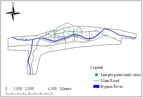
The research object of this paper is the land transfer price of residential land within the built-up area of QZ from 2013 to 2022. Through the website of the Bureau of Land and Resources and the website of the Ministry of Natural Resources of the People’s Republic of China, a total of 107 sample points of residential land grant price data within the built-up area in the 10-year period of 2013-2022 were collected, and the distribution of the sample points of land price is shown in Figure 2. The distribution of land price sample points is shown in Figure 2, in order to carry out the spatial and temporal evolution of residential land prices in the study area. The land price index of QZ urban area from 2013 to 2022 was obtained through the “China Land Price Monitoring Network”, and then the land price index was used to correct the collected residential land prices in the study area.

At the present stage, the land price index is based on a fixed-base index, i.e., the land price level of a fixed year in a specific area is used as the base index (usually recorded as 100), and then the land price of the subsequent years is comprehensively measured and compared with that of the base period to obtain the land price of the corresponding year. Land price monitoring uses a fixed-base index, which is modified by the formula shown in Eq. (17): \[\label{GrindEQ__17_} P=P_{0} *\frac{k_{0} }{k_{i} } , \tag{17}\] where \(P\) is the land price corrected to the base year, \(P\) is the actual transaction price of the land, \(k_{0}\) is the price index of the base year, and \(k_{i}\) is the land price index of the transaction year.

III. A. 3) Selection and quantification of factors affecting land prices

There are many factors that cause urban land prices to evolve in both spatial and temporal dimensions, and in the study targeting parcels of land, three main aspects are considered as micro-factors affecting the land prices of parcels of land, i.e., location factors, neighborhood factors, and individual factors of parcels of land. This study will select and quantify factors from these three aspects. Specifically, “urban main roads”, “key primary and secondary schools”, “large-scale shopping outlets”, “important bus stops “, “hospitals”, “parks”, “floor area ratio” and other seven influencing factors are included in the scope of investigation, and they are quantified separately. The quantified independent variables of the influencing factors are shown in Table 1.

Table 1 Quantification of the factors affecting the land price

Variable classes	Characteristic variable	Variable code	Variable quantification instructions	Unit
Location characteristics	Arterial road	ZGD	The nearest distance to the main road	m
Neighbourhood characteristics	School	XX	The closest distance to the school	m
	Large shopping	SH	Average distance from the last 3 major supermarkets	m
	Important bus stops	GJ	Distance from the nearest five key bus stops	m
	Hospital	YY	Distance from the nearest hospital	m
	Park green space	LD	Distance from the nearest park green space	m
Individual characteristics	Plot ratio	RJL	Upper limit of planned plot ratio	/

III. B. Exploratory spatial data analysis

III. B. 1) Analysis of spatial data structures

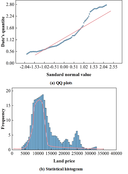
The spatial data structure analysis can explore the data distribution characteristics of urban land prices and analyze the distribution law of land price values. First, the land price data (corrected price by year) of 107 sample cities in the study area are statistically described, and the descriptive statistical analysis of urban land price in the study area is shown in Table 2. The spatial data distribution of land prices in the study area is shown in Figure 3(a) and (b) are the normal QQ plot and statistical histogram of land price data, respectively. The reference point of the normal QQ plot of land price data in the study area is obviously deviated from the straight line, indicating that the land price data do not obey normal distribution. The histogram of land price data shows that the distribution of land price data does not conform to the bell-shaped feature. Its skewness coefficient is positive (1.1795), indicating that there is a longer tail on the right side of the data distribution, and the kurtosis coefficient is 3.7852, indicating that the data distribution is steeper and more concentrated than the standard normal distribution. Therefore, the residential land price data needs to be transformed.

Table 2 Descriptive statistical analysis of urban land price

Number of samples	Minimum	Maximum	Mean	Standard deviation
107	4051.2	352241.8	12553	5875.49
Skewness	Kurtosis	First quartile	Median	Third quartile
1.1795	3.7852	8281	11521	15223

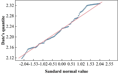
Using the Normal QQ Plot tool in ArcGIS to highlight the points that do not fall near the reference line in the QQ plot, the results show that there are two main types of data points that do not fall near the reference line. One is the data with lower values in the urban fringe area, and the other is the data with higher values in the main city area. The presence of lower or higher land values in the two areas caused the overall distribution of the data to not follow a normal distribution. \(\ln\) logarithmic transformation of the sample data, the normal distribution of the land price data after the logarithmic transformation is shown in Figure 4. At this time, the reference point of the QQ chart is closer to a straight line, indicating that the land price data after the logarithmic transformation is closer to obeying the normal distribution. This provides a basis for statistical interpolation of land price data.

III. B. 2) Trend analysis

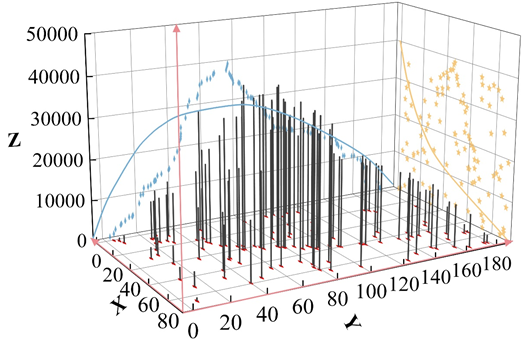
The trend of urban land prices in the study area was analyzed and the trend of land prices in the study area is shown in Figure 5, where the land price values were projected onto the horizontal and latitudinal planes respectively. The analysis of land price trend shows that in the X direction (horizontal trend), the land price data varies parabolically. Land prices first gradually increase from low to high along the inverted U-shaped curve until it reaches the apex located near the midpoint, and then it keeps decreasing along the U-curve. In the Y-direction (latitudinal trend), the data still follow the inverted U-shaped by line changes, but did not reach the apex in the study area, indicating that the land price shows a monotonous upward trend from the north to the south, and the slope change of the rising curve is small, which indicates that the rise is relatively stable.

The trend analysis reveals to some extent the changing trend of land prices in the study area. From west to east, i.e., from the urban fringe area gradually to the city center and its surroundings, land prices first rise and then fall, reaching a peak near the city center. After passing through the city center, land prices gradually decrease again from west to east. This shows that in the horizontal direction, land prices show a decreasing trend from the city center to the periphery. From the north to the south, land prices are generally climbing, with the rate of increase remaining generally stable.

III. B. 3) Spatial autocorrelation analysis

1. Global autocorrelation analysis

   Global spatial autocorrelation is to analyze the global autocorrelation of the data with Moran’ I index and use the standardized value of the test statistic for the significance test.The value domain of Moran’ I is [-1,1], if Moran’ I\(\mathrm{>}\)0,it means that the attribute characteristics X are positively correlated spatially, i.e. Land price level has similar attribute characteristics in neighboring regions, and the larger the value, the smaller the overall spatial difference. If Moran’ I\(\mathrm{<}\)0, it means that the attribute characteristics X space negative correlation that the land price level in adjacent regions have different attribute characteristics, and the larger the value, the larger the overall spatial difference, if Moran’ I=0, it means that the attribute characteristics space is not correlated, that is, the attribute characteristics of the land price level in the adjacent regions are independent of each other, in a random distribution. Table 3 shows the global autocorrelation analysis of land price. The Moran’ I index for all three time periods is greater than 0, indicating that the data are positively correlated. After obtaining the test statistic Z and the corresponding p, the values are compared with the significance level \(\alpha\) to determine the spatial autocorrelation among the observations (in a normal distribution, a confidence level of 0.05 threshold of 1.96 is generally chosen). Within the three time periods, the p-value is less than 1.96, based on the definition of the null hypothesis, then the null hypothesis does not hold, and the attribute characteristics are significantly positively correlated, i.e., the observed values show that the urban land prices are clustered for the high or low values of the same kind.

   Table 3 Global autocorrelation analysis of land price

   Project	2013\(\mathrm{\sim}\)2022	2013\(\mathrm{\sim}\)2017	2018\(\mathrm{\sim}\)2022
   Moran’ I index	0.4341156	0.297822	0.735518
   Expected index	-0.003019	-0.004383	-0.002985
   Variance	0.000589	0.001995	0.001088
   Z price	16.522483	6.852241	22.354681
   P price	0.000000	0.000000	0.000000

2. Local autocorrelation analysis

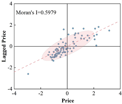
   The GeoDa spatial analysis tool was used to measure the local Moran’s I index of land prices in the study area, and the four quadrants of Moran’s scatterplot (I, II, III and IV) indicate “high-high autocorrelation”, “low-high autocorrelation”, “low-low autocorrelation”, and “high-low autocorrelation”, respectively. Figure 6 shows the local scatterplot of the study area, the Moran scatterplot shows that there are differences in the degree of correlation of land prices among the regions, with a z-value of 0.5979. Purely most of the regions have Local Moran’s I index in quadrants I and III, indicating that most of the study area land prices are positively correlated with their neighboring land prices (“high – high correlation” or “low – low correlation”). This indicates local autocorrelation of residential land prices in the study area. The area where the parcels are located with significance level greater than 0.05 is selected as the significant area of local autocorrelation and is highlighted in the Moran scatter plot. In this paper, both the local autocorrelation significance plot and LISA Cluster plot of land prices in the study area were obtained, indicating that there is a significant local autocorrelation phenomenon in a certain range of land prices in the study area, while the land prices in the remaining areas show a random distribution. The local autocorrelation analysis shows that the spatial correlation of land prices in the study area changes with location, i.e., the spatial dependence of land prices varies in different localized areas, which makes it necessary to spatially analyze the law of divergence of land prices.

III. C. Geostatistics-based analysis of spatial differentiation of land prices

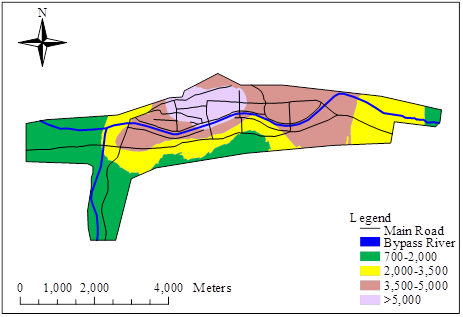
The spatial differentiation pattern of land price can reflect its spatial dependence and spatial heterogeneity phenomenon. Considering the spatial correlation of residential land prices in the study area and the fact that the number of sample points is not large enough and the spatial distribution is irregular, this paper adopts the kriging spatial interpolation method to interpolate the land price data. The study selected 107 pieces of residential land in the study area with corrected prices by year, preprocessed the data using logarithmic transformation, and applied kriging spatial interpolation to generate a continuous land price surface. Figure 7 shows the numerical model of land prices in the study area, which leads to the distribution pattern of land prices of residential land in QZ of TS city:

The spatial differentiation pattern of land prices in the study area shows a circle-to-circle decreasing pattern, which belongs to the monokernel spatial structure that gradually decreases from the center to the periphery, with jumping phenomenon in local areas. Land prices are generally higher in the peak land price area, which is the traditional business center of QZ, and the land price decreases slowly in the east-west direction and extremely fast in the north-south direction. Overall, the spatial differentiation pattern of land prices in the study area belongs to the “single-core” spatial structure that gradually decreases from the center to the periphery, and the land prices are spatially continuous with the CBD as the core of the city center to the periphery, and at the same time there are a few spatial variability phenomena, and the local conditions of the location of residential land have led to the presentation of the above spatial differentiation pattern of land prices. The localized location conditions of residential land have led to the above spatial differentiation pattern of land prices.

IV. Analysis of factors affecting the spatial differentiation of urban land prices

IV. A. Impact analysis of spatial differentiation of land prices based on LR modeling

The linear regression model expression is given below: \[\begin{aligned} \label{GrindEQ__18_} Y_{i} =&6331.7552-3.2285X_{ZGD} -0.1601X_{XX} +0.4771X_{GJ} -1.5502X_{YY} \notag \\ &{-0.5233X_{SH} -0.3245X_{LD} -2.1596RJL}. \end{aligned} \tag{18}\]

Let the land value of the \(i\)th sample point be \(Y_{i}\), \(X_{ZGD}\), \(X_{XX}\), \(X_{GJ}\), \(X_{YY}\), \(X_{SH}\) and \(X_{LD}\) represent the closest distance from the land value sample point to the urban arterial road, school, public transportation station, hospital, life service facilities and urban green space respectively. \(RJL\) represents the plot ratio of a land price sample point. Table 4 shows the parameter estimates of the linear regression model. The regression coefficients and significance tests of the linear regression model were analyzed with the following results:

1. The distance from hospitals and urban green space is negatively correlated with land price, in which the regression coefficient of “distance from hospitals” is -1.5502, with a p-value of less than 0.05, which indicates that the land price of residential land is significantly negatively correlated with the distance from hospitals, and the land price of residential land decreases significantly with the increase of the distance from hospitals. The regression coefficient of “distance to green space” is -0.3245, which indicates that the closer the residential plots are to the urban green space, the higher the price is within the study area.

2. Except for the factor of “distance to public transportation station”, which has a positive relationship with residential land price, all other factors have negative regression coefficients, which is in line with the expectation. However, half of the regression coefficients have a P-value as high as 0.5, which indicates that the correlation between these factors and residential land price is not significant enough.

Table 4 Linear regression model parameter estimation

Serial	Influencing factor	Regression coefficient	Standard error	T	P
0	Constant		499.5123	12.8551	0.0000
1	\( X_ZGD \)	-3.2285	2.4456	-1.4456	0.0894
2	\( X_XX \)	-0.1601	0.6223	-0.2883	0.8021
3	\( X_GJ \)	0.4771	1.1528	0.4513	0.6558
4	\( X_YY\)	-1.5502	0.5337	-2.8314	0.0044
5	\( X_SH \)	-0.5233	0.6889	-0.7618	0.3838
6	\( X_LD \)	-0.3245	0.2789	-1.1578	0.0255
7	\( RJL\)	-2.1596	165.3852	-0.0145	0.9895

IV. B. Impact analysis of spatial differentiation of land prices based on GWR modeling

The GWR model requires that the nature of the data’s self-contained coordinates can be well integrated with GIS to visualize the results of GWR calculations and make the description of the data easier and clearer.

IV. B. 1) GWR Modeling

Let the \(i\)st sample point land price is \(y_{i}\), \(x_{ik}\) represents the closest distance from the land price sample point to an influential factor, and \(\beta\) represents the regression coefficient of the factor, then the GWR model can be constructed as Eq. (19): \[\begin{aligned} \label{GrindEQ__19_} y_{i} =&\beta _{0} \left(u_{i} ,v_{i} \right)+\beta _{iZGD} \left(u_{i} ,v_{i} \right)x_{i1} +\beta _{iXX} \left(u_{i} ,v_{i} \right)x_{i2} +\beta _{iGJ} \left(u_{i} ,v_{i} \right)x_{i3} +\beta _{iYY} \left(u_{i} ,v_{i} \right)x_{i4} \notag \\ &{+\beta _{iSH} \left(u_{i} ,v_{i} \right)x_{i5} +\beta _{iLD} \left(u_{i} ,v_{i} \right)x_{i6} +\beta _{iRJL} \left(u_{i} ,v_{i} \right)x_{i7} +\varepsilon _{i} } \notag\\ =&\beta _{0} \left(u_{i} ,v_{i} \right)+\sum _{k=1}^{7}\beta _{k} \left(u_{i} ,v_{i} \right)x_{ik} +\varepsilon _{i}. \end{aligned} \tag{19}\]

In the formula, \(\beta _{iZGD}\), \(\beta _{iXX}\), \(\beta _{iGJ}\), \(\beta _{iYY}\), \(\beta _{iSH}\), \(\beta _{iLD}\), \(\beta _{iRJL}\) represent the regression coefficients of the influence degree of urban main roads, the influence degree of schools, the influence degree of bus stops, the influence degree of hospitals, the influence degree of living services, the influence degree of urban green space and the influence degree of the floor area ratio at \(i\) points, with the coefficient uniformly \(\beta _{ik}\), and the seven coefficients are written into the summation formula, so as to simplify the formula.

IV. B. 2) GWR model calculations

Simulation estimation using geographically weighted regression model, the first to determine the form and method of distance weighting and bandwidth, this study in the process of experimental comparison and analysis, the final use of Gaussian-like distance Bi-square function, AIC method validated by the adaptive bandwidth calculation method, optimized bandwidth distance of 1921.45m.

The advantage of regression analysis in the GWR model is that each residential sample point land price has a corresponding regression coefficient. Table 5 shows the descriptive statistics of the contribution of 107 land price influencing factors, which are mainly selected as Minimum (Min), Upper Quartile (Q1), Median (Median), Lower Quartile (Q3), Maximum (Max), Mean (Mean), and Standard Deviation (S). Table 6 shows the results of Monto Carlo test for significance. The standard deviation (S) value can be used to determine the dispersion of the contribution of each influence factor, the larger the standard deviation of an influence factor, the more obvious the spatial differentiation. In the table, the volume ratio has the largest regional difference in the contribution of residential land price. From the mean (Mean) of all the influencing factors, floor area ratio and public transportation stations have a greater impact on residential land price. Among them, the marginal effect of volume ratio on residential land price reaches 122.5385 Yuan/m², which reflects the importance of volume ratio on residential land price. The smaller the plot ratio means that the floor will be lower, high-rise general plot ratio is larger, high-rise generally need to configure the elevator, for ordinary residents, the higher the floor of the common share will also increase accordingly, so ordinary residents hope that the plot ratio is smaller. In order to intensively and efficiently utilize land resources, the government has certain restrictions on the plot ratio of industrial and commercial land, which reflects the necessity of macro-control. The factor of main road reflects the traffic condition of the study area, from the table we can see that the marginal force of the main road on the residential land price is 3.1362 Yuan/m², and the distance from the main road is shortened by 1km, and the residential land price rises by 3136.2 Yuan, which reflects that the convenient transportation can enhance the urban residential land price to a certain extent. From the significance probability value p in the Monto Carlo test significance table, there is a large regional difference in the contribution of main roads, schools, hospitals and volume ratio to residential land price.

Table 5 Descriptive statistics of GWR model calculation results

Parameter	Min	Q\(\_1\)	Median	Q\(\_3\)	Max	Mean	S
Intercept	3873.32	5265.41	6061.29	6726.50	7312.49	5898.98	928.95
D-ZGD	-6.5386	-5.0107	-4.1366	-2.1446	4.6564	-3.1362	2.6974
D-XX	-2.1882	-0.696	0.0324	0.245	1.4253	-0.2954	0.9007
D-DJ	-1.7898	-0.1021	0.4522	1.0644	2.3889	0.4718	0.864
D-YY	-3.0454	-2.5582	-2.1929	-1.3136	0.2589	-1.8208	0.9578
D-SH	-1.2632	-0.9151	-0.2869	0.1584	1.975	-0.2977	0.6823
D-LD	-2.5056	-0.5659	-0.3715	-0.2812	-0.0178	-0.5246	0.4687
RJL	-197.550	111.9701	140.5295	179.8499	232.0199	122.5385	89.6968

Table 6 Significance after Monto Carlo test

Parameter	P	significance level
Intercept	0.0000	***
D-ZGD	0.0048	**
D-XX	0.0355	*
D-DJ	0.4552	n/s
D-YY	0.0388	*
D-SH	0.1665	n/s
D-LD	0.1261	n/s
RJL	0.0018	***

IV. C. Impact of various influencing factors on land prices in the study area

The GWR model focuses on local characteristics, and the regression coefficients of each factor can be obtained through geographically weighted regression. Applying the Kriging spatial interpolation method to interpolate the regression coefficients and visualize the spatial changes of the regression coefficients facilitates the in-depth analysis of the impact of land price influencing factors on the land price of the local area.

1. Influence of main roads on residential land prices

   The influence of main roads on residential land prices in this study is shown in Figure 8. From the measured values of the regression coefficients of the GWR model for the road factors, the regression coefficients range from -6.511 to 4.522, of which only 14.95% (16) of the regression coefficients are positive, and the rest are negative. The closer to the main highway, the higher the residential land price, and the closer to the main highway, the lower the land price. The area to the east is close to the highway, with more noise pollution and environmental pollution, so combining these factors indicates that in these areas the main road has a positive effect on land prices.

   

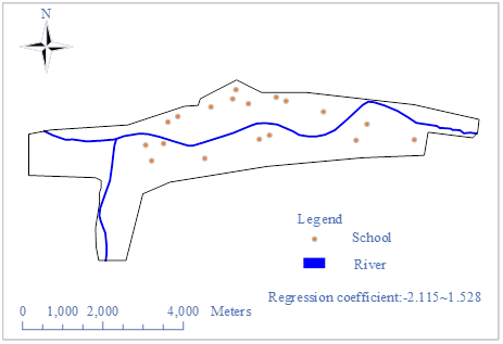
2. Impact of Schools on Residential Land Prices

   The influence of school on residential land price is shown in Figure 9. From the regression coefficient of the factor “distance to school”, the regression coefficient ranges from -2.115 to 1.528, among which 46.73% (50/107) of the land prices increase with the decrease of distance to school. The areas with negative correlation between “distance to school” and land price are mainly located near the east of the city, which have fewer schools and lack of better educational resources, and a good humanistic environment has a great influence on the residents of the neighboring areas in choosing their residences, and since the city center and the vicinity of the Teachers’ College itself have high-quality educational resources, and the distribution of primary and middle schools is more even, the sensitivity of schools to land price starts to be higher in these areas. Schools are starting to become less sensitive to land prices.

   

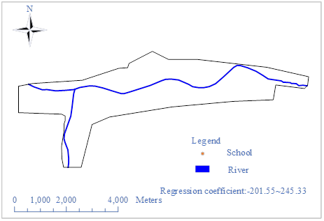
3. Relationship between plot ratio and land price

   The impact of volume ratio on residential land price is shown in Figure 10. From the measured value of the regression coefficient of the GWR model for the factor of floor area ratio, the range is -201.55\(\mathrm{\sim}\)245.33, which shows that the floor area ratio has a significant impact on the residential land price, and the highest marginal impact value can be up to 245.33 yuan/square meter. A large number of high-rise buildings are distributed in the area near the busy district, which is the main commercial center, so there are more high-rise buildings with larger plot ratios, and the residential land prices in this area are also higher.

V. Conclusion

Based on the existing theory of spatial differentiation of land prices, this paper puts forward the concept of spatial differentiation of urban land prices, and through the empirical research on the residential market in QZ city, it proactively explores the pattern of spatial differentiation of land prices by combining spatial analysis with spatial statistical analysis, and analyzes the correlation between land prices and their influencing factors by building a geographically-weighted regression model to analyze the causes of spatial differentiation of residential land prices in the city. Through theoretical and empirical research, the following main conclusions are obtained:

1. The data of residential land price sample points in the study area basically conforms to normal distribution, with land price showing a U-shape in the latitudinal direction, and land price in the horizontal direction, with land price showing a gradual decline from the city center to the periphery. From the north to the south, the land price is generally climbing up, and the rise remains stable in general. At the same time, there is a “single core” spatial structure that gradually decreases from the center to the periphery, and the land price expands spatially in a continuous manner with the CBD as the core of the city center to the periphery in a continuous manner, with a few spatial variability phenomena at the same time.

2. The model results show that the GWR model is better than the general linear regression model, and from the regression results of the GWR model, individual factors of the land \(\mathrm{>}\) location factors \(\mathrm{>}\) neighborhood factors. There are large locational differences in the contribution of plot ratio, distance from main roads, distance from hospitals and distance from schools to residential land price, among which the marginal effect of plot ratio on residential land price reaches 122.5385 yuan/m², reflecting the importance of plot ratio to residential land price.

Funding

2024-2026 Young Talent Support Project of China Association for Agricultural Machinery Institute, Research on the development strategy of intelligent Agricultural equipment in Sichuan Province (2022JDR0359), Research on the innovative development strategy of agricultural equipment Industry in hilly and mountainous areas of Jiangxi Province (2024-02JXZD-01).