
With the rapid development of China’s national economy, the scale of infrastructure is expanding, and the available land for construction is getting tighter and tighter, occupying a large number of open areas that do not meet the foundation bearing capacity requirements [1]. The use of special treatment to strengthen the existing natural site has become an indispensable measure to improve the strength of the foundation, to ensure the stability of the foundation [2,3]. In foundation engineering, the study of soil dynamic properties is crucial to the building safety and stability of the project [4]. In order to minimize unforeseen disasters, it is necessary to carry out experimental tests for foundation soils in advance and to analyze the corresponding soil properties in order to take the necessary precautions in the construction project [5-7]. In addition, if the construction treatment of foundation foundation and pile foundation cannot be carried out reasonably, it will also reduce the stability of the building foundation structure and adversely affect the construction quality of the overall project [8-10]. For the soil dynamic characteristics in the construction of foundation foundation and pile foundation of construction project, the construction enterprise should focus on combining the characteristics of the foundation structure and the situation, formulate a perfect construction technology program, strengthen the application of foundation construction technology, ensure that the stability and strength of the overall foundation structure is in accordance with the standard, and consolidate the foundation for the smooth progress of the construction of building project [11-13].
The quality control of foundation construction is very important for civil engineering, and the use of stable foundation treatment techniques can ensure the construction control results. Literature [14] took a 20-story building as an experimental object and used the elasto-plastic nonlinear ontological model of soil to numerically study and time domain three-dimensional nonlinear dynamic analysis of its soil-structure interaction (SSI) effects, and the results pointed out that the foundation deformation capacity has a certain proportionality with the maximum foundation shear (seismic demand), and with the foundation’s rigidity of the rotational relationship. Literature [15] constructed a detailed three-dimensional numerical model of a full-size reinforced concrete structure based on soil-structure interaction effects in order to investigate the nonlinear dynamic response of reinforced concrete structures in depth, and the results showed that SSI can cause changes in the nonlinear dynamic response of the RC frame. Literature [16] investigated the structure-soil-structure interactions of adjacent buildings with base-isolated buildings and buildings with conventional reinforced concrete frame structures, and it was found through numerical and soil model simulation experiments that the response acceleration of the base-isolated buildings was more than four times lower than that of the conventional buildings for the same seismic response. Literature [17] proposed an algorithm for testing and calculating the dynamic stability of sandy soils and conducted experimental tests using a medium-sized natural quarry sand as an example, and the results verified the effectiveness of the proposed algorithm to qualitatively and quantitatively assess the behavior of unconnected soils under dynamic loading.
Meanwhile, literature [18] emphasized the importance of soil-structure interaction and used two methods, the nonlinear Beam of Winker Method (BNWM) and direct soil modeling, to analyze the soil-structure interaction effects in the seismic vulnerability analysis of concrete buildings. Literature [19], after analyzing the performance characteristics of buildings in loess and loess areas, used numerical analysis and shaking table model test methods to explore the dynamic response law of high steep loess slopes under building loads and seismic loads, and then to derive the safety distance of buildings at the top of the slope to maintain the structural stability of the buildings. Literature [20] pointed out the relationship between the efficiency of foundation isolation and the dynamic properties of the system and the site response spectrum, and explored the influence mechanism between soil-structure interaction and the dynamic response of high-rise buildings in foundation isolation by a method applicable to non-classically damped systems, and the results showed that foundation isolation has an inhibiting effect on the effects of deleterious soil-structure interaction. Literature [21], after discussing the influence mechanism between dynamic soil-structure interaction and the effects of building structures, gives the main assessment methods of seismic soil-structure interaction problems as well as the commonly used modeling techniques and computational methods, which will provide a theoretical basis for future in-depth research in the field of SSI.
The study, based on the calculation of stability and three-dimensional finite element model, takes the student teaching building of a college in city A as an example, and analyzes the supporting structure of its foundation pit building construction from the effects of soil moisture content, different seismic levels on the role of different clays. Then indoor experiments were carried out to study the contact characteristics of different clays and slate foundation floors, and then an earthquake-resistant structural joint action model was established to verify the different clays as the main holding layer from static and dynamic aspects, and to explore the analysis of the seismic effects of earthquakes on clays. The feasibility of adopting clay soil building foundations is investigated to provide reference for similar construction projects.
Spectral analysis is actually the combination of the results of modal analysis and statistically calculated spectra to calculate the response of the structure, such as displacement and stress analysis means, here the response spectral curve, in fact, is the statistics of different single-mass elastic structural system in the earthquake under the maximum response and the structure of the self-oscillation period and get, that is, the response and the period of a kind of correspondence between the response and the period, and they are all in the stages of conformity with a certain kind of They all conform to a certain functional relationship at each stage.
Response spectrum analysis is based on the theory of response spectrum of vibration mode decomposition, the so-called vibration mode decomposition is actually the structure in the seismic action of various responses, such as displacement, acceleration, etc., as the structure of the superposition of the components of each vibration mode, which is equivalent to each vibration mode has a result, and then through a number of mathematical statistics of the combination of the structural response of each vibration mode under the superposition, we can get the result of each vibration mode. The total seismic response of the structure is obtained by superposition of the seismic response under each vibration mode by some combination of mathematical statistics (SRSS, CQC, ABS, etc.). The calculation procedure is as follows.
Equations of motion for a multi-degree-of-freedom system are: Inertial forces: \[\label{GrindEQ__1_} I_{i} =m_{i} \left(\ddot{x}_{t} +\ddot{x}_{g} \right) . \tag{1}\] Elastic Resilience: \[\label{GrindEQ__2_} S_{i} =k_{i1} x_{1} +k_{i2} x_{2} +\cdots k_{in} x_{n} . \tag{2}\] Damping force: \[\label{GrindEQ__3_} R_{i} =c_{n} \dot{x}_{1} +c_{i2} \dot{x}_{2} +\cdots c_{in} \dot{x}_{n} . \tag{3}\] Equations of motion: \[\label{GrindEQ__4_} m_{i} \ddot{x}_{i} +\sum _{j=1}^{n}c_{ij} \dot{x}_{i} +\sum _{j=1}^{n}k_{ij} x_{i} =-m_{i} \ddot{x}_{g} . \tag{4}\] \[\label{GrindEQ__5_} \left[m\right]\left\{\ddot{x}\right\}+\left[c\right]\left\{\dot{x}\right\}+\left[k\right]\left\{x\right\}=-\left[m\right]\left\{I\right\}\ddot{x}_{g} \left(t\right) . \tag{5}\]
For a multi-degree-of-freedom system, take a two-degree-of-freedom linear system for example, and superimpose the displacements \(x_{1} (t)\) and \(x_{2} (t)\) of the primes \(m_{1}\) and \(m_{2}\) with a linear superposition, i.e: \[\label{GrindEQ__6_} \left. \begin{array}{l} {x_{1} (t)=q_{1} (t)X_{11} +q_{2} (t)X_{21} } \\ {x_{2} (t)=q_{1} (t)X_{12} +q_{2} (t)X_{22} } \end{array}\right\} . \tag{6}\]
Chinese codes use different methods of analysis according to the type and height of the house and the flat elevation arrangement of the structure. Since the analysis of reaction is more mature, it is used as the main design method in most countries.
The theoretical expression for the structural motion of time course analysis is as follows: \[\label{GrindEQ__7_} \left[M\right]\left\{\ddot{U}\right\}+\left[C\right]\left\{\dot{U}\right\}+\left[K\right]\left\{U\right\}=P\left(t\right) , \tag{7}\] where \(\left[M\right]\) – is the mass matrix of the structure, \(\left[C\right]\) – is the damping matrix of the structure, \(\left[K\right]\) – is the stiffness matrix of the structure, \(\left\{\ddot{U}\right\}\left\{U\right\}\left\{\dot{U}\right\}\) – are the acceleration, displacement, and velocity vectors of the structure, respectively and \(P\left(t\right)\) – the excitation due to loads or seismic waves.
A potential problem in the stepwise integration of the response of a multi-degree-of-freedom system is that the damping matrix must be defined directly without using the vibration damping ratio, and estimating the magnitude of the damping influence coefficients for the entire damping matrix is very difficult [22]. In general, the most efficient way to derive a damping matrix is to assume appropriate damping ratios for the full range of vibration shapes that have significant effects, and then compute an orthogonal damping matrix with those properties. We will discuss the incremental expression of the integral equation again below.
In the analysis of a multi-degree-of-freedom system, the incremental equilibrium equations are derived by taking the difference between the vector equilibrium relational equations determined at moments \(t_{0}\) and \(t_{1} =t_{0} +h\): \[\label{GrindEQ__8_} \Delta f_{I} +\Delta f_{D} +\Delta f_{S} =\Delta p . \tag{8}\]
The increment of the force vector can be expressed as: \[\label{GrindEQ__9_} \Delta f_{l} =f_{l_{1} } -f_{l_{2} } =m\Delta \dot{v} , \tag{9}\] \[\label{GrindEQ__10_} \Delta f_{D} =f_{D_{1} } -f_{D_{0} } =C_{0} \Delta \dot{v} , \tag{10}\] \[\label{GrindEQ__11_} \Delta f_{S} =f_{S_{1} } -f_{S_{0} } =k_{0} \Delta v , \tag{11}\] \[\label{GrindEQ__12_} \Delta p=p_{1} -p_{0} . \tag{12}\]
Substituting the four Eqs. of (12) into (13), the incremental equation of motion becomes: \[\label{GrindEQ__13_} m\Delta \ddot{v}+c_{0} \Delta \dot{v}+k_{0} \Delta v=\Delta p . \tag{13}\]
The structure deforms under the action of load, if the load remains in equilibrium after the deformation, we call it elastic equilibrium. If the structure in equilibrium is subjected to a force that causes the structure to deviate from its previous equilibrium position, and when the force disappears the structure can be brought back to its previous equilibrium state, we call this a stable equilibrium state, and if the force is withdrawn after the force is applied and the structure is still not able to be brought back to its previous equilibrium state, we call this an unstable equilibrium state [23]. If we apply a certain load to the structure and add a small increment on top of that, and the shape of the structure changes a lot, this is the case that the structure is destabilized or the structure is buckled, and that certain load is the buckling load of the structure.
Currently, there are two types of buckling analysis: linear buckling analysis and nonlinear buckling analysis, ANSYS provides eigenvalue buckling analysis.
Now we present eigenvalue buckling analysis.
In the stable equilibrium state described in the previous subsection, the equilibrium equation of the structure is: \[\label{GrindEQ__14_} \left(\left[K_{E} \right]+\left[K_{G} \right]\right)\left\{U\right\}=\left\{P\right\} . \tag{14}\]
The structure reaches casual equilibrium, and the second-order variant of its system potential energy should be 0, i.e., \[\label{GrindEQ__15_} \left(\left[K_{E} \right]+\left[K_{\sigma } \right]\right)\left\{\delta U\right\}=0 . \tag{15}\]
Therefore there must be: \[\label{GrindEQ__16_} \left|\left[K_{E} \right]+\left[K_{G} \right]\right|=0 . \tag{16}\]
Assuming a set of loads \(\left\{P^{0} \right\}\) with its corresponding geometric stiffness matrix of \(\left\{K_{G}^{0} \right\}\), and assuming that the load in buckling is \(\lambda\) times that of \(\left\{P^{0} \right\}\), then (16) reduces to: \[\label{GrindEQ__17_} \left|\left[K_{E} \right]+\lambda \left[K_{G}^{0} \right]\right|=0 . \tag{17}\]
Transformed into the following equation: \[\label{GrindEQ__18_} \left(\left[K_{E} \right]+\lambda _{i} \left[K_{G} \right]\right)\left\{\phi _{i} \right\}=0 , \tag{18}\] where \(\lambda _{i}\) is the \(i\)nd order eigenvalue: \(\left\{\phi _{i} \right\}\) is the deformed shape of the structure, called the buckling mode of the structure.
Said above, the source of seismic action is the building structure to maintain the original state will produce this inertia of the force, the size of this force is changed with the seismic wave intensity, seismic wave intensity is also changed with time, in the calculation of this force we usually use the integral method, the formula is: \[\label{GrindEQ__19_} F=mS_{o} =Mg\frac{\left|\bar{x}_{0} (t)\right|}{g} \frac{S_{o} }{\left|\bar{x}_{0} (t)\right|} =k\beta G . \tag{19}\]
In case \(\alpha =k\beta\), the elastic system of a single mass point with degrees of freedom under the action of a horizontal earthquake is expressed as follows: \[\label{GrindEQ__20_} F=\alpha G . \tag{20}\]
A building structure with an irregular plan layout will torsion during an earthquake. At this time the effect produced by the action is as follows:
The formula for determining the standard value of the \(i\)nd floor of the \(j\)st vibration mode under horizontal seismic action is: \[\label{GrindEQ__21_} \left. \begin{array}{c} {F_{xji} =\alpha _{i} \gamma _{tj} X_{ji} G_{i} } \\ {F_{yji} =\alpha _{i} \gamma _{tj} Y_{ji} G_{i} } \\ {F_{zji} =\alpha _{i} \gamma _{tj} r^{2} \varphi _{ji} G_{i} } \end{array}\right\}\left(i=1,2,\cdots ,n;j=1,2,\cdots ,m\right) \tag{21}\] where \(F_{xji}\), \(F_{yji}\), \(F_{sji}\) are the standard value of seismic action in the \(x\)-direction, \(y\)-direction and corner direction of the \(j\)-vibration type \(i\) layer, respectively, \(X_{ji}\), \(Y_{ii}\) are \(j\) vibration type \(i\) layer of the center of mass in the \(x\), \(y\) direction horizontal relative displacement, \(\varphi _{ji}\) is \(j\) vibration mode \(i\) layer relative torsion angle, \(r_{i}\) is radius of rotation of layer \(i\), which can be taken as the positive quadratic root of the ratio of the moment of inertia of rotation of layer \(i\) around the center of mass to the mass of this layer, \(\alpha _{i}\) is seismic response parameters corresponding to the self-oscillation period \(T_{j}\) of the \(j\)th vibration mode, \(\gamma _{tj}\) is the parameters of vibration mode \(j\) considering torsion, \(n\) is the calculated total number of masses of the structure and \(m\) is the total number of vibration modes calculated for the structure.
Considering the unidirectional horizontal seismic action in case of structural torsion, the action effect can be determined by the following formula: \[\label{GrindEQ__22_} S=\sqrt{\sum _{j=1}^{m}\sum _{k=1}^{m}\rho _{\mu } S_{j} S_{k} } , \tag{22}\] \[\label{GrindEQ__23_} \rho _{jk} =\frac{8\zeta _{j} \zeta _{k} \left(1+\lambda _{T} \right)\lambda _{T}^{1.5} }{\left(1-\lambda _{T}^{2} \right)^{2} +4\zeta _{j} \zeta _{k} \left(1+\lambda _{T} \right)^{2} \lambda _{T} } , \tag{23}\] where \(S\) is the torsion of the standard value of seismic effects, \(S_{j}\), \(S_{k}\) are the standard value of seismic effects for vibration modes \(j\) and \(k\) respectively, \(\rho _{jk}\) is the coupling coefficients for \(j\) and \(k\) vibration modes, \(\lambda _{T}\) is the self-oscillating period ratio for vibration modes \(k\) and \(j\), respectively and \(\zeta _{j}\), \(\zeta _{k}\) are the damping ratio for vibration modes \(j\) and \(k\), respectively.
The standard value of seismic action shear force at each level of the structure is satisfied when calculating the horizontal seismic action: \[\label{GrindEQ__24_} V_{EKi} \ge \lambda \sum _{j=i}^{n}G_{j} , \tag{24}\] where \(V_{Eki}\) is the shear force at the \(i\)nd floor corresponding to the standard value of horizontal seismic action, \(\lambda\) is the horizontal seismic shear coefficient, \(G_{j}\) is the representative value of gravity load on the \(j\)th floor and \(n\) is the total number of floors of the building structure.
Discretization of structure
Segmentation of a continuous elastomer results in a fixed number of units with a fixed shape. The process of transforming a continuum split like this into the combined form of a fixed number of units is called discretization [24]. After discretization, it is assumed that the units are connected only by nodes, i.e., the nodes play the role of force transmitters between the units and the neighboring units. There is a marvelous relationship between units and elements and so on units they are connected to each other and need to have some parameter or bond to connect them with each other so that the role of points can be reflected. In any type of finite element method calculation, the primary means, the first step is discretization.
Selection of the displacement interpolation function
The second step of the finite element method is to select the displacement interpolation function, the displacement of the unit depends on the displacement of the nodes, while the overall stress and strain is usually determined by the displacement of the nodes, so in order to make the final solution convergence, the interpolation function to meet the displacement continuity conditions, but also to meet the conditions of constant strain [25]. Usually in the analysis can be summarized in each unit node displacement summarized into a kind of easy to understand function, expressed in polynomials, the choice of this function should be that is simple and appropriate and reasonable, the results of finite element analysis will be accurate.
The matrix function is: \[\label{GrindEQ__25_} \left\{f\right\}=\left[N\right]\left\{\delta \right\}^{e} , \tag{25}\] where \(\left\{f\right\}\) is the displacement of any point in the cell, \(\left\{\delta \right\}\) is the displacement of the node of the cell and \(\left[N\right]\) is the line function.
Analyze the mechanical properties of the unit
First, the unit strain is described by the node displacements: \[\label{GrindEQ__26_} \left\{\varepsilon \right\}=\left[B\right]\left\{\delta \right\}^{e} , \tag{26}\] where \(\left\{\varepsilon \right\}\) is the strain of the unit and \(\left[B\right]\) is the matrix of unit strains.
Using the equation of the intrinsic relationship, the unit stresses are also presented in terms of nodal displacements: \[\label{GrindEQ__27_} \left\{\sigma \right\}=\left[D\right]\left[B\right]\left\{\delta \right\} , \tag{27}\] where \(\left[D\right]\) is the elasticity matrix related to the unit material.
Finally, according to the variational principle, the equation of the relationship between the forces at the nodes of the unit and the resulting displacements (i.e., the equilibrium equation) is derived: \[\label{GrindEQ__28_} \left[F\right]=\left[K\right]^{e} \left\{\delta \right\}^{e} , \tag{28}\] where \(\left[K\right]\) is the unit stiffness matrix \[\label{GrindEQ__29_} \left\{k\right\}=\int \int \int \left[B\right]^{T} \left[D\right]\left[B\right]dxdydz . \tag{29}\]
Superimpose the unit equilibrium equations to derive the equilibrium equations for the continuum (i.e., the total stiffness matrix \(\left[K\right]\)): \[\label{GrindEQ__30_} \left[K\right]=\sum \left[K\right]^{e} . \tag{30}\]
The overall equilibrium equations are introduced from the total stiffness matrix: \[\label{GrindEQ__31_} \left[K\right]\left\{\delta \right\}=\left[F\right] . \tag{31}\]
This section takes the example of a college student teaching building project at the intersection road of Architecture Avenue and Guangming Road in City A, and analyzes the soil quality, geological profile, and seismicity level impacts on and during the construction of the building project.
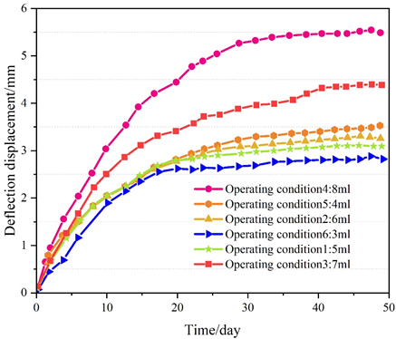
In the calculation process, the deformation characteristics of the support structure on the side near the river are mainly analyzed. Soil water content change working conditions are taken: increase and decrease, respectively. The changes of soil water content in specific calculation conditions are shown in Table 1. From Table 1, it can be seen that the soil water content of working conditions 2\(\mathrm{\sim}\)4 shows a growing trend, which increased by 6 ml, 7 ml and 8 ml, respectively, while the working conditions 5\(\mathrm{\sim}\)7 start to decrease, and the soil water content of each working condition decreased by 4 ml, 3 ml and 2 ml, respectively.
| Operating condition | Water content | Operating condition | Water content |
| Operating condition 1 | Water content 5ml | Operating condition 5 | Reduced water volume 4ml |
| Operating condition 2 | Increment 6ml | Operating condition 6 | Reduced water volume 3ml |
| Operating condition 3 | Increment 7ml | Operating condition 7 | Reduced water volume 2ml |
| Operating condition 4 | Increment 8ml |
The lateral displacement curve with time at the top of the adjacent pit support is shown in Figure 1. From Figure 1, it can be seen that the test displacement develops with time, first increasing and then stabilizing. The seasonal change of soil moisture content has some influence on the foundation pit support structure; when the soil moisture is normal, the cumulative lateral displacement is about 3.2mm; with the increase of soil moisture content, the lateral displacement of the support structure gradually increases, and when the moisture content grows to 7 ml and 8 ml, the cumulative values of lateral displacement are 4.4mm and 5.5mm, which are increased by 1.2mm and 2.3mm, respectively, with an increase of 37.50% and 71.88%; dry period to reduce the soil water content, to a certain extent, alleviate the lateral pressure of the support structure, calculations show that the lowering of the amount of water to support the lateral displacement of the structure change is small, mainly due to the soil nails support and the soil body of the tensile force between the role. It shows that the rainy season should be avoided when carrying out building construction.
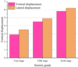
It has been proposed that the construction of the foundation pit project tries to avoid the rainy season as much as possible, therefore, only the normal soil water content is considered for the stability analysis of the support structure affected by earthquakes. At the same time, considering that City A is a 4-degree zone, the probability of sudden large earthquakes is small, and only 4, 5 and 6 grade earthquakes are considered for analysis. The calculation results of the displacement of the top of the support with time for different earthquake levels are shown in Figure 2.
From Figure 2, it can be seen that: with the increase of seismic grade, the lateral displacement and vertical settlement gradually increase, but the increase is not large; the lateral displacement at seismic grade 4, 5 and 6 is 3.5mm, 4.9mm and 6.2mm respectively, and the value-added is 1.4mm and 1.3mm; the vertical displacement at seismic grades 4, 5 and 6 is 2.9mm, 4.5mm and 5.8mm, and the value-added is 1.6mm and 1.3mm in order; and the value-added is 1.6mm and 1.6mm in order. is 1.6mm and 1.3mm in order.
In summary, it can be seen that: the soil water content increases the lateral displacement of the supporting structure becomes larger, but the amplitude of the increase in the amount of water and the amplitude of the increase in the lateral displacement does not show a corresponding development, indicating that the higher the soil water content not only to consider the lateral additional stress, but also to consider the penetration of water on the soil softening effect. Therefore, the pit building construction tries to avoid the summer vacation rainfall period. In proposing the basis of pit building construction try to avoid the summer season with abundant rainfall, so only the normal soil moisture content is considered in the analysis of the stability of the support structure affected by the earthquake. The deformation of the support structure increases with the increase of seismic level, but considering the low seismicity of City A, the impact of earthquake on the support structure is controlled within the range of 4mm, which is relatively small, and it can also be said that increasing the seismic level appropriately will have less impact on the support structure of the foundation pit.
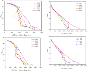
The results of floor shear and bending moment internal force calculations are shown in Figure 3. As can be seen from Figure 3: the specification of the time-range analysis results require that the structure are bottom shear and vibration mode decomposition reaction spectrum method than the result is not less than 1; each seismic wave bottom shear and reaction spectrum than the result is not less than 0.72, from the above analysis can be obtained from the above time-range analysis results can satisfy the specification requirements; through the comparison of the above internal force curve graphs can be obtained, each seismic wave elastic time-range analysis of the floor shear and the floor overturning bending moment and the results of the reaction spectrum is basically close to the safety assessment. By comparing the above internal force curves, it can be seen that the floor shear and floor overturning moment of each seismic wave elastic time course analysis are basically close to the results of the reaction spectrum of the safety assessment, and the floor shear of individual seismic wave is larger than the results of the reaction spectrum of the safety assessment in some floors.
After the calculation is completed, the vertical stresses and settlements on the surface of the soil body at each level are extracted, and the vertical stresses and settlements of the soil body are shown in Table 2.
From Table 2, it can be seen that the stresses on the soil body increase sequentially from top to bottom, and on the same horizontal plane, there is a significant difference in the magnitude of the stresses on the soil body due to the different distances from the building. Fill and coarse sand layer are less stressed due to the existence of excavation area, as the main bearing layer of foundation 3 clay, the average value of vertical stress on its surface is 266.08kPa, which is much smaller than the characteristic value of foundation bearing capacity of 498kPa, so the bearing capacity meets the requirements.
In terms of settlement in each layer, the greater the thickness of the soil layer, the greater the settlement. In the soil layer below the raft foundation, the maximum settlement difference within the layer is greater than that of the surface soil. The average settlement of the soil layer below the foundation is 69.45mm, and the total settlement of the whole foundation soil is 76.23mm. According to Article 5.3.4 of Code for the Design of Building Foundation GB50007-2011, for the towering structure with Hg\(\mathrm{\le}\)100m, the maximum foundation deformation allowable value is 402mm, therefore, it meets the specification requirements.
| Soil layer | Vertical stress (kPa) | Layer settlement (mm) | |||||
| Minimum | Maximum | Average | Minimum | Maximum | Average | Maximum sedimentation difference | |
| 1 Soil packing | 16.71 | 35.25 | 25.37 | 4.22 | 6.23 | 5.44 | 2.22 |
| 2 Coarse sand | 52.11 | 157.35 | 99.13 | 2.05 | 3.41 | 2.02 | 0.92 |
| 3 Clay | 82.06 | 719.65 | 266.08 | 21.21 | 44.71 | 29.22 | 24.32 |
| 4 Powdered clay | 334.05 | 698.04 | 574.55 | 8.55 | 15.45 | 11.04 | 7.23 |
| 5 Clay | 416.67 | 726.44 | 618.33 | 20.75 | 37.25 | 29.21 | 18.11 |
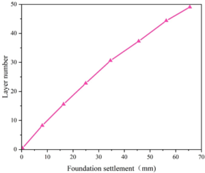
In order to simulate the change rule of foundation soil settlement during construction, the original analysis step was adjusted to activate the gravity of the superstructure and the floor panel load every 4 floors to extract the settlement of the soil surface of the holding layer below the midpoint of the footing, and the change of the foundation settlement with the floor load is shown in Figure 4. It can be seen that the rate of foundation soil subsidence increases with the increase of floor loads, from 0 at the beginning until it approaches 50.
The results of vertical stress and single layer settlement extracted from 3 clay layer under different gradation are shown in Table 3.
From Table 3, it can be seen that in the simulation results of four kinds of grading soil samples, the settlement of grading 3 is the largest, and the vertical stress suffered by grading 2 is the largest, with a force value of 83.33. In both the settlement and force, the well-graded grading 1 is smaller than that of the poorly-graded grading 2. In addition, comparing the grading 1, 3, 4, it can be found that, in the case of the equal values of Cu and Cc, the larger the largest particle size, the larger the average stress and settlement suffered by clay is also larger. Stress and settlement is also greater. The maximum settlement difference within the layer follows a similar pattern, increasing with the increase in the maximum grain size of the clay, and is smaller for well-graded clays than for poorly graded clays.
Therefore, it can be concluded that, all other conditions being equal, the use of well-graded clay soil foundation with fine grain size can reduce the settlement and settlement difference of foundation soil to a certain extent and improve the bearing performance.
| Grading | Vertical stress (kPa) | Layer settlement (mm) | |||||
| Minimum | Maximum | Average | Minimum | Maximum | Average | Maximum sedimentation difference | |
| Grading 1 | 82.23 | 714.41 | 267.12 | 19.65 | 45.23 | 28.21 | 27.41 |
| Grading 2 | 83.33 | 745.33 | 282.56 | 19.81 | 47.75 | 29.1 | 28.76 |
| Grading 3 | 82.43 | 783.13 | 281.77 | 18.57 | 47.24 | 31.32 | 29.32 |
| Grading 4 | 82.13 | 704.65 | 276.44 | 19.13 | 46.56 | 29.11 | 28.32 |
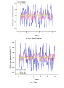
After the calculation is completed, the horizontal acceleration, velocity and displacement of each layer of soil surface directly below the center point of the foundation are extracted, and the results are shown in Figures 5-7 below.
Horizontal acceleration
It can be seen that the acceleration of the soil layer is getting smaller and smaller with the increase of depth, and the fluctuation is getting smoother and smoother. The acceleration waveform on the surface of clay 1 is basically the same as the input original wave, with amplitudes of 37.29 cm/s² and 281.45 cm/s², respectively, which are decreased compared with the amplitude of the original wave. The reason is that there is a joint action between the building slab and the soil layer at the wave source, and the input surface wave is transmitted to the stiff superstructure through the foundation, causing the superstructure to exert a reverse force on the surface, so that the actual seismic response of the subgrade soil is weakened.
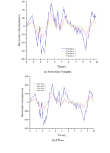
Horizontal velocity
Similar to the acceleration time-course curve, the velocity of the clay layer gradually slows down with increasing depth, and the fluctuation tends to be smaller and smaller. The maximum velocity on the surface of Clay 1 under the 8\(\mathrm{{}^\circ}\) multiple-occurrence earthquake is 67.22 mm/s, while that under the rare-occurrence earthquake is 523.55 mm/s, which is a 7.8-fold difference. It can also be noticed that the peak velocity points of each clay layer appear almost simultaneously, but the time of appearance is slightly postponed as the clay layer goes downward.
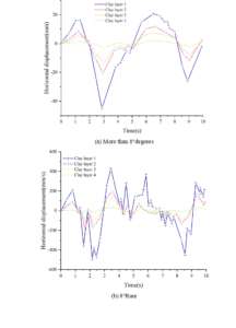
Horizontal displacement
Under the action of 8\(\mathrm{{}^\circ}\) multiple and rare earthquakes, the displacement of the soil body becomes smaller and smaller with the depth, and the thicker the soil layer that the seismic wave passes through, the greater the degree of attenuation of its displacement, and the degree of attenuation of the displacement of the rare seismic wave propagated to the surface of clay 2 through clay 1 is obviously greater than that of the multiple earthquakes, and the maximum velocity on the surface of clay 1 under the rare earthquakes is 483.35 mm/s, while that of the surface of clay 1 under the multiple earthquakes is 44.6 mm/s. This indicates that the seismic performance of this clay foundation is better than that of the small earthquakes. This indicates that the seismic performance of this clay foundation is better in large earthquakes than in small earthquakes.
This paper firstly takes the construction of a teaching building for students of a college in city A as an example, introduces the calculation method of this paper into the stability analysis of foundation pit support structure, constructs the hierarchical model of the factors affecting the stability of the building support structure, and analyzes the effects of building stability, soil water content and different seismic grades on different soil qualities. With the increase of soil water content, the lateral displacement of the supporting structure becomes larger, and the increase of soil water content and lateral displacement do not have mutual influence on the development. It shows that the more the soil water content should not only consider the lateral additional force, but also consider the penetration softening effect of water on the soil. Therefore, foundation pit building construction should try to avoid the rainy season. The effect of earthquake on the supporting structure is controlled within 4mm, which is relatively small, indicating that an appropriate increase in seismicity level has a small effect on the supporting structure of foundation pit building.
Subsequently, the structural co-action model was constructed to study the contact characteristics of clay on the building ground for some of the academic floors of the college. The results show that the maximum foundation settlement and overall inclination of clay 1 under static loading under structural co-action is less than the code limit, while the maximum surface velocity of clay 1 under rare earthquakes is 483.35 mm/s, while the maximum surface velocity of clay 1 under multiple earthquakes is 44.6 mm/s. This indicates that the seismic performance of this clay foundation is better during large earthquakes than during small earthquakes.