Research on Utility Analysis and Risk Prediction of Economic Management of Construction Enterprises in Digital Economy

I. Introduction

As the digitalization process of the construction industry continues to accelerate, the enterprise economic management mode is also more and more intelligent, informatization and digitalization, which effectively enhances the competitiveness of the enterprise market and ensures that the enterprise meets the challenges of economic globalization in a better posture. Based on this, analyzing the utility of economic management of construction enterprises, as well as studying the related risk prediction methods, can provide certain reference for the economic management and development of enterprises in the construction industry.

The construction process of construction projects covers engineering budgets, resource deployment, organizational structure and other management contents related to the economy [1,2]. Strengthening the control of the relevant management content in the engineering project can, on the one hand, guarantee the connection between different departments in the enterprise and promote the communication and exchange between departments [3-5]. It can also scientifically and reasonably adjust all kinds of resources in the project, strengthen the balance of the enterprise in the management work, so as to realize the reasonable allocation of resources in the enterprise, and support the enterprise as much as possible to achieve the goal of the expected results [6-9]. However, in the actual operation of the enterprise, the economic management is still affected by a variety of factors, such as direct economic losses caused by material waste, indirect economic losses caused by untimely deployment of personnel, etc. [10,11]. Only by correctly analyzing the utility of the enterprise’s economic management behavior in the work, and researching the related risk prediction scheme, can we further improve the enterprise’s economic management mode and lay a solid foundation for the good development of the enterprise [12,13].

Literature [14] puts forward the numerical analysis method in the enterprise economic management, by analyzing and processing the numerical problems of the enterprise economy, it effectively solves the defects of poor prediction accuracy and low management efficiency that exist in the traditional economic and economic management model. Literature [15] designs a computerized visual signature encryption system based on RSA algorithm and MD5 message digest algorithm, which guarantees the security and confidentiality of digital signatures of enterprise economic contracts. Literature [16] develops a new type of economic analysis system based on cloud computing for small and medium-sized enterprises (SMEs), which meets the needs of SMEs for the computational and storage capacity of economic statistical systems, and improves the quality of monitoring services while significantly reducing the cost of business information and communication. Literature [17] uses a deep learning model to carry out risk analysis, revenue analysis, and profit and loss analysis of the behavior of economic activities and the financial indicator system in enterprise management, and formulates relevant strategies for the development of the enterprise’s financial economy based on the visualized financial and economic data map. Literature [18] shows that the information management system helps enterprises to maintain timely and effective communication with the market, and the implementation of information management can improve the quality and management level of the enterprise, so based on the financial situation of the enterprise, a set of neural network algorithm based on the financial management of the cloud platform system is designed. Literature [19] introduces Markov model to optimize the enterprise financial management system, which is often used for economic condition prediction due to its dynamic adaptability and high demand for data, and experiments have proved that the model improves the efficiency of financial resource allocation. Literature [20] explains the necessity of developing the digital capability of enterprise financial management and proposes to use visual recognition algorithms to visualize the features of enterprise financial management system to enhance its financial risk identification, assessment and control functions.

According to the theory of digital economy and economic management of construction enterprises, the utility and risk evaluation index system of economic management of construction enterprises in digital economy is constructed. With the help of information entropy theory, the weight value of the utility evaluation indexes of construction enterprise economic management is calculated, and the utility of construction enterprise economic management is comprehensively evaluated. The construction enterprise economic management risk indicators as the number of neurons in the input layer of the BP neural network model, based on the model simulation and verification analysis, the number of hidden layer, the model output layer for five risk levels (very low risk, lower risk, general risk, higher risk, very high risk), and finally determine the number of nodes in the input layer of the model is 21, the number of nodes in the hidden layer is 100, and the number of nodes in the output layer is 5. Using the model of this paper, the evaluation of the utility and risk evaluation system of construction enterprise economic management is carried out. The model of this paper to predict and analyze the economic management risk of construction enterprises. The innovation of this paper is that instead of establishing a judgment matrix, data normalization is used to quickly calculate the weighting results.

II. Study of the utility of economic management in construction enterprises

II.A. Effectiveness evaluation indicator system

In the context of digital economy and sustainable development, high technology and globalization features significantly, the construction industry has shown a fierce competitive situation with many competitors and diverse competitive situations [21]. In the construction process of construction projects, it covers project budget, resource deployment, organizational structure and other economy-related management content. It can be seen that the economic management of construction projects is a systematic, process-oriented, closed-loop all-round management work, the bargaining power of the building construction enterprises to suppliers and buyers is weakening year by year, and the cost pressure and business risks are rising. This paper stands from the perspective of sustainable development of construction enterprises, puts forward the evaluation index system construction principles, and then determines the utility evaluation index system of construction enterprise economic management.

II.A. 1) Principles for the construction of the price indicator system

On the basis of the theory of sustainable development of construction enterprises, the construction of construction enterprises’ economic management utility evaluation index system needs to satisfy the principles of objectivity and fairness, and the principle of dynamics, which are described as follows:

1. The principle of objectivity and fairness, the objectivity and fairness of the source and basis of the evaluation index system of the economic management of construction enterprises, the objectivity of the process and method of evaluating the economic management of construction enterprises, and the reliability and objectivity of the evaluation results.

2. The principle of dynamism: the evaluation index system of the economic management utility of construction enterprises should not only be compatible and integrated with the economic management objectives of the construction enterprises, reflecting and promoting the economic management utility of the construction enterprises, but also be adapted to the fluctuating changes of the huge uncertainty of the internal and external environment of the enterprises.

II.A. 2) Determination of the system of evaluation indicators

The evaluation index system of economic management utility of construction enterprises is shown in Table 1. Under the requirements of the principles of objectivity and impartiality and the principle of dynamism, the evaluation index system of economic management utility of construction enterprises is finalized, which consists of 7 first-level indexes (Profitability Q1, Solvency Q2, Survivability Q3, Cost Management Efficiency Q4, Capital Management Ability Q5, and Organizational Operational Efficiency Q6, human capital management Q7) and 20 secondary indicators (return on investment Q11, net profit margin Q12, static payback period Q13, financial net present value Q14, internal rate of return Q15, interest provision ratio Q21, debt service provision ratio Q22, gearing ratio Q23, current ratio Q24, quick ratio Q25, net cash flow from operations Q31, accumulated surplus funds Q32, cost Control Q41, Cost Forecasting and Planning Q42, Access to Funds Q51, Financial Risk Control Q52, Financial Accountability Q61, Enterprise Management System Q62, Talent Selection and Training Q71, International Perspective and Continuing Education Q72).

Table 1 Enterprise economic management utility evaluation index system

Primary index	Symbol	Secondary index	Symbol
Profitability	Q1	Investment yield	Q11
		Net profit rate	Q12
		Static investment recovery period	Q13
		Net present value	Q14
		Internal rate of return	Q15
Solvency	Q2	Interest payment rate	Q21
		Repayment rate	Q22
		Asset ratio	Q23
		Mobility ratio	Q24
		Speed ratio	Q25
Viability	Q3	Operating net cash flow	Q31
		Accumulated surplus fund	Q32
Cost management efficiency	Q4	Cost control	Q41
		Cost forecast and plan	Q42
Capital management capability	Q5	Capital acquisition	Q51
		Financial risk control	Q52
Organizational efficiency	Q6	Economic responsibility	Q61
		Enterprise management system	Q62
Human capital management	Q7	Talent selection and culture	Q71
		International vision and continuing education	Q72

II.B. Evaluation index weights based on information entropy

After determining the utility evaluation index system of the economic management of the construction enterprise, the information entropy method is applied immediately afterward to calculate the numerical size of its weight, and the detailed calculation principle and process are shown below:

II.B 1) Information entropy theory

After eliminating the scale and normalizing the evaluation matrix, we get the calculation matrix \(Y\), where \(0\le y_{ij} \le 1\); assuming that a reasonable weight matrix \(P\) has been established for the evaluated indexes, \(p_{j}\) represents the weight of the \(j\)th evaluation index [22]. Obviously, for the weight matrix after normalization, conditions \(\sum p_{j} =1\) and \(p_{j} \ge 0\) should be satisfied, in order to determine the weight matrix \(P\), we should construct a function \(H\) of the computational matrix \(Y\). According to the nature of the weights, we can obtain the properties of the function \(H\) and the relevant interpretation of these properties.

1. Symmetry: \(H(x_{1} ,x_{2} )=H(x_{2} ,x_{1} )\). When the order of the evaluation object is changed, the weight of the same evaluation index should remain unchanged, i.e., any two rows of the calculation matrix \(Y\) are changed, and the function value should remain unchanged.

2. Monotonicity: when the evaluation indicators are more important in the evaluation system, the function value obtained should be larger. In particular, if there is only one evaluation indicator, then its weight is 1, then the corresponding function \(H\) should be able to take the maximum value. It should be noted that, although the theoretical requirements of the function \(H\) has a monotonically increasing nature, but in the construction of the function does not need to be reflected, we can be corrected at a later stage of a decreasing number of drawings.

3. Continuity: when the number of evaluation objects to determine the function of its variables \(y_{1} +y_{2}\) should have continuity, which can ensure that the final weight coefficient has good computational properties.

4. Additivity: when \(x_{2} =y_{1} +y_{2}\), then \(H(x_{1} ,y_{1} ,y_{2} )=H(x_{1} ,x_{2} )+x_{2} H\left(\frac{y_{1} }{x_{2} } ,\frac{y_{2} }{x_{2} } \right)\). When an evaluation object is divided into two additive parts, then the original function \(H\) should have the weighted sum property. (Obviously, this additivity is not a linear relationship.)

Based on the above four principles, we can construct the function, which can be obtained: \[\label{GrindEQ__1_} H\left(x_{1} \cdots x_{n} \right)=-c\sum _{i=1}^{n}x_{i} \ln x_{i} . \tag{1}\]

Here \(c\) is the normalization factor, the logarithm of the bottom of the \(e\) is taken for the sake of simplicity, and does not affect the final results of the calculation, the only problem is that \(H(x_{i} \cdots x_{n} )\) is monotonous subtractive function is not consistent with the custom. Therefore, after the calculation, the deviation must be calculated for trimming. And formula (1) and the definition of information entropy is the same, so we can use information entropy to calculate the weights. For function \(H(x_{1} \cdots x_{n} )=-c\sum _{i=1}^{\pi }x_{i} \ln x_{i}\) when satisfy \(x_{n} =y_{1} +y_{2}\), there is: \[\label{GrindEQ__2_} H(x_{1} \cdots x_{n-1} ,y_{1} ,y_{2} )=H(x_{1} \cdots x_{n} )+x_{2} H\left(\frac{y_{1} }{x_{2} } ,\frac{y_{2} }{x_{2} } \right) . \tag{2}\] Available \[\begin{aligned} \label{GrindEQ__3_} H(x_{1} \cdots x_{n-1} ,y_{1} ,y_{2} )&=-c\left(\sum _{i=1}^{n-1}x_{i} \ln x_{i} +y_{1} \ln y_{1} +y_{2} \ln y_{2} \right)\notag \\ &{=-c\sum _{i=1}^{n}x_{i} \ln x_{i} -cx_{n} \left(\ln y_{n} -\frac{y_{1} }{x_{n} } \ln y_{1} -\frac{y_{2} }{x_{n} } \ln y_{2} \right)}\notag\\ &{=H(x_{1} \cdots x_{n} )+x_{n} H\left(\frac{y_{1} }{x_{n} } ,\frac{y_{2} }{x_{n} } \right)}. \end{aligned} \tag{3}\]

II.B. 2) Weighting process

First the data matrix \(X\) is normalized to obtain the computational matrix \(Y\), which can be obtained: \[\label{GrindEQ__4_} y_{ij} =\frac{x_{ij} -\bar{x}_{*j} }{\max x_{*j} -\min x_{*j} } , \tag{4}\] where \(\max x_{\bullet j} ,\min x_{\bullet j} ,x_{\bullet j}\) represents the maximum value, minimum value and average value of column \(j\) of data matrix \(X\), respectively. Because the entropy value as the calculation of weights does not evaluate the actual entropy value (information) of a certain evaluation index, but reflects the role of the corresponding evaluation index in the given evaluation system and the relative importance of the evaluation index. From the point of view of information theory, it represents the degree of useful information in the problem, so the way of processing the data matrix \(X\) does not reduce the amount of information carried by the data itself. Therefore we can define the normalization formula (4) according to the problem to be evaluated.

Calculate the entropy value. According to formula (1), we can calculate the entropy value of each evaluation indicator. Where the entropy value of the \(j\)th indicator is: \[\label{GrindEQ__5_} H_{j} =-\frac{1}{\ln n} \sum _{ij}^{n}a_{ij} \ln a_{ij} . \tag{5}\] The sign is taken here because the entropy value is guaranteed to be positive and the normalization factor is defined as \(c=\frac{1}{\ln n}\).

Calculate the value of evaluation index weights as: \[\label{GrindEQ__6_} w_{j} =\frac{1-H_{j} }{n-\sum _{j=1}^{m}H_{j} } \tag{6}\] changing monotonicity while normalizing.

II.C. Economic management utility evaluation model

II.C. 2) Establishment of a rubric

A rubric set refers to a collection of various overall evaluations of the likelihood of a project’s level of risk, generally denoted by the capital letter \(V\), i.e. [23]: \[\label{GrindEQ__7_} V=\{ V_{1} ,V_{2} ,\cdots ,V_{n} \}. \tag{7}\]

II.C. 2) Designing the questionnaire and creating the weight set

1. Questionnaire design

   Evaluate the single-factor risk and establish the fuzzy relationship matrix \(R\), i.e., adopt the method of experts filling in the questionnaire to score, collect the evaluation of each risk factor \(r_{ij}\) by the experts, and establish the corresponding fuzzy relationship matrix \(r(r_{ij} )\): \[\label{GrindEQ__8_} r_{ij} =\frac{{\text {For a single risk factor, experts divide people into a certain class}}}{{\text{ Number of reviewers}}}. \tag{8}\] The fuzzy relationship matrix \(r\) is obtained: \[\label{GrindEQ__9_} r=\left[\begin{array}{ccccc} {r_{11} } & {r_{12} } & {r_{13} } & {…} & {r_{1n} } \\ {r_{21} } & {r_{22} } & {r_{23} } & {…} & {r_{2n} } \\ {…} & {…} & {…} & {…} & {…} \\ {r_{m1} } & {r_{m2} } & {r_{m3} } & {…} & {r_{mn} } \end{array}\right] . \tag{9}\]

2. Establishment of weight set

   The weight set reflects the different levels of importance of each risk factor, i.e., the relative importance of each risk factor as determined earlier in the information entropy theory, and the set consisting of these weight vectors: \[\label{GrindEQ__10_} W=\{ w_{1} ,w_{2} ,\cdots ,w_{m} \} \quad a_{i} (i=1,2,\cdots \cdots ,m) . \tag{10}\]

   Known as the factor weight set, referred to as the weight set []. The determination of the weight set is a very important part of the comprehensive evaluation of project risk, assuming that the same risk factors, the selection of different weights, the final evaluation results will be very different. Fuzzy comprehensive evaluation based on hierarchical analysis will undoubtedly greatly improve the accuracy of project risk evaluation.

II.C. 3) Fuzzy integrated evaluation

The evaluation matrix synthesis in the fuzzy comprehensive evaluation method usually adopts the method of “weighted average” to synthesize the fuzzy comprehensive evaluation matrix in a hierarchical manner. The weight matrix \(W_{i}\) and the fuzzy judgment matrix \(r\) are synthesized to get the fuzzy comprehensive evaluation matrix \(R\). The specific addition method is as follows: \[\label{GrindEQ__11_} R=W_{i} *r=(w_{1} ,w_{2} ,…,w_{m} )*\left[\begin{array}{ccccc} {r_{11} } & {r_{12} } & {r_{13} } & {…} & {r_{1n} } \\ {r_{21} } & {r_{22} } & {r_{23} } & {…} & {r_{2n} } \\ {…} & {…} & {…} & {…} & {…} \\ {r_{m1} } & {r_{m2} } & {r_{m3} } & {…} & {r_{mn} } \end{array}\right] . \tag{11}\]

The fuzzy comprehensive evaluation result vector \(B\) is obtained by synthesizing the weight matrix \(W\) with the evaluation matrix \(R\), which can be obtained: \[\label{GrindEQ__12_} B=W*R=W*\left[\begin{array}{c} {R_{1} } \\ {R_{2} } \\ {R_{3} } \\ {…} \\ {R_{n} } \end{array}\right] . \tag{12}\]

The final risk level of the project is then determined based on the principle of maximum affiliation.

II.D. Utility analysis of economic management in construction enterprises

II.D. 1) Calculation of evaluation indicator weights

The initial data is derived from a construction economic website, and the weights of the utility evaluation indicators of the economic management of construction enterprises are calculated according to the calculation formula and principles mentioned in subsection 2.3, and the results of the evaluation indicator weights are shown in Figure 1. According to the numerical performance in the figure, it can be seen that the order of the weights of the first-level indicators is Q25 (0.0752) \(\mathrm{>}\) Q13 (0.0721) \(\mathrm{>}\) Q51 (0.0721) \(\mathrm{>}\) Q15 (0.0690) \(\mathrm{>}\) Q23 (0.0690) \(\mathrm{>}\) Q11 (0.0683) \(\mathrm{>}\) Q22 (0.0606) \(\mathrm{>}\) Q32 (0.0560) \(\mathrm{>}\) Q61 (0.0560) \(\mathrm{>}\)Q71 (0.0552) \(\mathrm{>}\)Q52 (0.0414) \(\mathrm{>}\)Q72 (0.0414) \(\mathrm{>}\)Q21 (0.0391) \(\mathrm{>}\)Q62 (0.0391) \(\mathrm{>}\)Q41 (0.0360) \(\mathrm{>}\)Q31 (0.0330) \(\mathrm{>}\)Q12 (0.0284) \(\mathrm{>}\)Q24 (0.0284) \(\mathrm{>}\)Q14 (0.0230), and the second-level indicator weights are ranked as follows Q2 (0.2722)\(\mathrm{>}\)Q1 (0.2607)\(\mathrm{>}\)Q5 (0.1135)\(\mathrm{>}\)Q7 (0.0966)\(\mathrm{>}\)Q6 (0.0951)\(\mathrm{>}\)Q3 (0.0891)\(\mathrm{>}\)Q4 (0.0729), and also the size of the symbols in the graph can be discerned by the index weight ordering. A comprehensive overview of the size of the utility evaluation index weights of the economic management of construction enterprises is provided to provide data support for the following comprehensive evaluation and analysis.

II.D. 2) Comprehensive evaluation analysis

The frequency of evaluation of economic management utility of construction enterprises is shown in Table 2. According to the set of rubrics, the economic management utility of construction enterprises is divided into five grades, which are excellent, good, average, poor, and poor, respectively, to complete the set of rubrics \(V=\left\{v_{1} ,v_{2} ,v_{3} ,v_{4} ,v_{5} \right\}\), and the five rubrics are assigned the value of 5, 4, 3, 2, and 1. In order to realize the analysis of the evaluation of the economic management utility of the construction enterprises, a certain construction enterprise is selected as a research object, and the 10 experts in the field of construction assess the grade of the research object, and the combination of above The weights, the comprehensive evaluation formula and the principle of maximum affiliation can be derived from the results of the analysis of the economic management utility evaluation of construction enterprises.

Table 2 Economic management utility evaluation frequency

Secondary index	Symbol	Excellence	Good	General	Passing	Difference
Investment yield	Q11	5	3	1	1	0
Net profit rate	Q12	3	4	1	1	1
Static investment recovery period	Q13	4	3	0	0	3
Net present value	Q14	4	4	2	0	0
Internal rate of return	Q15	4	4	1	1	0
Interest payment rate	Q21	3	4	1	1	1
Repayment rate	Q22	4	4	2	0	0
Asset ratio	Q23	3	3	0	1	3
Mobility ratio	Q24	3	2	1	1	3
Speed ratio	Q25	4	2	1	0	3
Operating net cash flow	Q31	4	4	1	0	1
Accumulated surplus fund	Q32	4	3	2	1	0
Cost control	Q41	4	3	2	1	0
Cost forecast and plan	Q42	4	3	2	1	0
Capital acquisition	Q51	4	3	2	0	1
Financial risk control	Q52	4	3	1	0	2
Economic responsibility	Q61	4	4	2	0	0
Enterprise management system	Q62	5	4	1	0	0
Talent selection and culture	Q71	4	3	2	1	0
International vision and continuing education	Q72	5	3	1	1	0

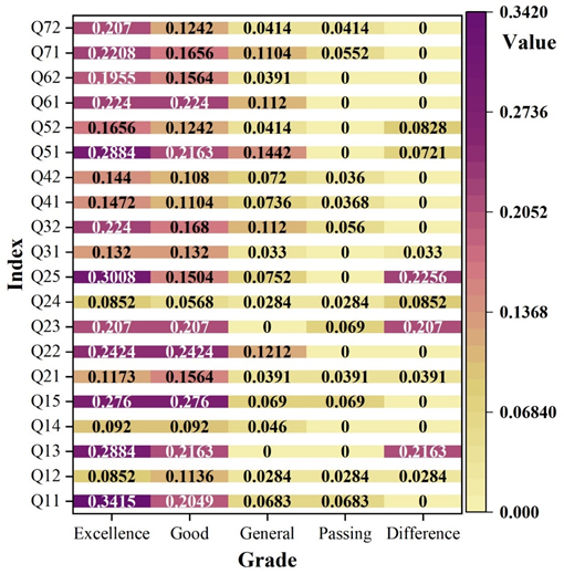
The weight matrix \(W_{i}\) and the fuzzy judgment matrix \(r\) are synthesized to get the fuzzy comprehensive evaluation matrix \(R\), and the fuzzy comprehensive evaluation matrix is shown in Figure 2. According to the data in Figure 2, while combining the principle of maximum affiliation degree, the comprehensive evaluation of the economic management utility of construction enterprises can be obtained: \[B=W*R=W*\left[\begin{array}{c} {R_{1} } \\ {R_{2} } \\ {R_{3} } \\ {…} \\ {R_{n} } \end{array}\right]=\left[3.9843,3.2449,1.2547,0.5276,0.9895\right].\] Based on the comprehensive evaluation results of the economic management utility of the construction enterprise [3.9848, 3.2449, 1.2547, 0.5276, 0.9895], it is summarized that the economic management utility of the construction enterprise is in an excellent position, and it has an important guiding value for the promotion of the sustainable development of the construction industry.

III. Forecasting risks in the economic management of construction companies

III. A. Principles for the selection of risk indicators

III. A. 1) Systemic principles

In the systematic principle, the evaluation index system required to be constructed is studied from a global perspective, which can form a unified level in time and form a specific and comprehensive reflection of the level of economic management risk of the whole construction enterprise.

III. A. 2) Scientific principles

When establishing the construction enterprise economic management risk evaluation index system, it is necessary to use scientific and reasonable assessment methods. At the same time, there should be a certain theoretical support, and the risk indicator system is easy to understand and grasp, only all these issues will be taken into account to determine the risk system of economic management of construction enterprises, in order to ensure that it can be effectively used in the subsequent research.

III. A. 3) Principle of independence

Due to the connection between various factors, or the similarity of the meaning of more than two elements, it is difficult to distinguish them, so the principle of independence is to ensure the consistency of the indicators, while the principle of independence is to divide the functions and functions of the indicators well, and each element should accurately reflect a factor, so as to reduce the crossover of the indicators. The independence of the indicators is guaranteed.

III. A. 4) Principle of testability

In the process of developing the risk evaluation system, the existing evaluation system should be tested by applying scientific methods, and the impact of which should be preliminarily screened and verified, so that only the factors that have been screened and retained can become the criteria for evaluation.

III. B. System of indicators for evaluating economic management risks

The construction enterprise economic management risk evaluation index system is shown in Table 3, synthesizing the relevant resources in this field and the principles of evaluation index system construction, and finally determining the construction enterprise economic management risk evaluation index system, which consists of 7 first-level indicators and 14 second-level indicators.

Table 3 Economic management risk evaluation index system

Primary index	Symbol	Secondary index	Symbol
Strategic risk	R1	Market competitiveness	R11
		Industry policy change	R12
Market risk	R²	Market demand fluctuation	R²1
		Industry policy change	R²2
Investment risk	R3	Return on project investment	R31
		Chain stability	R32
Operational risk	R4	Production efficiency	R41
		Human resource stability	R42
Financial risk	R5	solvency	R51
		Liquidity risk	R52
Legal risk	R6	Contract performance risk	R61
		Intellectual property risk	R62
Project management risk	R7	Project extension risk	R71
		Engineering quality control	R72

III. C. Risk prediction models

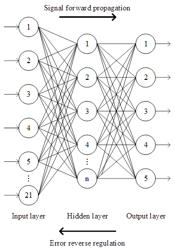
BP neural network generally adopts three-layer structure, and the three-layer network has better information processing function and learning ability, which is able to fit any function and provide feedback and adjustment on the discrepancy between input and output at any time. Therefore, this paper proposes to construct a three-layer BP neural network for economic management risk prediction of construction enterprises.

III. C. 1) BP neural networks

Learning of BP neural network consists of two phases, the first phase is forward propagation through input signals and the second phase is back propagation through errors [25].

The structure of the BP neural network is shown in Figure 3, and the basic implementation steps of the BP algorithm are as follows:

1. Initialize the weights and thresholds of the network.

2. Given a set of network training sample set.

3. Calculate the output values of the implicit and output layers based on the formula.

   The output of the hidden layer is: \[\label{GrindEQ__13_} al_{i} =f1\left(\sum _{j=1}^{r}\omega l_{ij} p_{j} +bl_{i} \right) . \tag{13}\]

   The output of the output layer is: \[\label{GrindEQ__14_} a2_{k} =f2\left(\sum _{i=1}^{s1}\omega 2_{ki} al_{i} +b2_{k} \right) . \tag{14}\]

4. Adjust the connection weights and thresholds of the network. \[\label{GrindEQ__15_} x(k+1)=x(k)+\alpha D(k) . \tag{15}\]

5. Calculate the total error of the neural network: \[\label{GrindEQ__16_} E=\frac{1}{2} \sum _{k=1}^{s2}(t_{k} -a2_{k} )^{2} . \tag{16}\]

6. Cycle through steps 2 through 3 until the error accuracy satisfies \(\varepsilon\), i.e., \(E<\varepsilon\).

III. C. 2) Determination of the number of nodes in each layer

1. Number of nodes in the input layer

   Based on the economic management risk indicators of construction enterprises described in subsection 3.2, the number of neurons in the input layer of the BP neural network model, which is also the number of economic management risk indicators of construction enterprises, is derived, which is 21 in total (of which there are 7 first-level indicators and 14 second-level indicators), which are strategic risk R1, market risk R², investment risk R3, operational risk R4, financial risk R5, legal risk R6 project management risk R7, market competitiveness R11, industry policy change R12, market demand fluctuation R²1, industry policy change R²2, project return on investment R31, capital chain stability R32, production efficiency R41, human resource stability R42, solvency R51, liquidity risk R52, contract fulfillment risk R61, intellectual property rights risk R62, project extension risk R71, project quality control R72, these 21 indicators as the input layer nodes of the BP model.

2. Number of implicit layer nodes

   The complexity of the structural model of BP neural network is closely related to the number of nodes in its hidden layer. In order to prevent the number of neurons in the hidden layer from being too many or too few, and at the same time to ensure the generality and performance of the network, based on the existing research, we suggest adding 1-2 neurons to accelerate the reduction of the error rate under the given conditions, and using a compact structure as much as possible. Gradually increase the number according to the results of training, compare the errors and find out the optimal number of neurons to get the optimal number of neurons; another method is that, use some empirical formulas to calculate, the empirical formulas are as follows: \[\label{GrindEQ__17_} m=\sqrt{n+l} +a , \tag{17}\] \[\label{GrindEQ__18_} m=\log _{2} n , \tag{18}\] \[\label{GrindEQ__19_} m=\sqrt{nl} , \tag{19}\] \[\label{GrindEQ__20_} m=\frac{n+l}{2} . \tag{20}\]

3. Number of nodes in the output layer

   The risk classification relationship is shown in Table 4, and the most common method of BP neural network in multi-classification problems is solved by setting \(n\) output node. In this paper, the risk is classified into five categories: very low risk, low risk, average risk, high risk, and very high risk before the assessment and prediction. So in this paper, these five features are used as the output, and it is enough to design the output variable as a five-dimensional vector, and use it as the output, which results in the number of neuron nodes in the output layer as 5.

Table 4 Risk classification relation

Expectancy classification	Risk classification	The five dimensional vector
1	Low risk	[1,0,0,0,0]
2	Lower risk	[0,1,0,0,0]
3	General risk	[0,0,1,0,0]
4	High risk	[0,0,0,1,0]
5	Very high risk	[0,0,0,0,1]

III. D. Selection of the excitation function

The main role of excitation function in BP neural network is to convert the input signal into output signal. Usually, the commonly used excitation functions in neurons are categorized into the following three types:

1. Threshold function, denoted as: \[\label{GrindEQ__21_} f(x)=\left\{\begin{array}{l} {0,\qquad\qquad x<0}, \\ {1,\qquad\qquad x\ge 0}.\end{array}\right. \tag{21}\] \[\label{GrindEQ__22_} f(x)=\left\{\begin{array}{l} {-1,\qquad\qquad\;\; x<0}, \\ {\;\;1,\qquad\qquad \;\;\;x\ge 0}. \end{array}\right. \tag{22}\]

2. The segmented linear function, denoted as \[\label{GrindEQ__23_} f(x)=\left\{\begin{array}{ll} {-x,} & {x\le 0} \\ {cx,} & {0<x<x_{c} } \\ {\;\;x,} & {x\ge 0}. \end{array}\right. \tag{23}\]

3. S(Sigmoid) type function, denoted as \[\label{GrindEQ__24_} f(x)=\frac{1}{1+e^{-x} } . \tag{24}\]

   The S-type excitation function is shown in Figure 4, compared with the threshold and segmented linear excitation function, the S-type excitation function is microscopic, simple to compute and easy to express, and it also has a very good performance of nonlinear mapping, which can compress all the values of the inputs between (-1, 1), and has a nonlinear amplification function. So S(Sigmoid) type function is used in this study.

III. D. 1) Loss function

The LogLoss log loss function is also known as the cross-entropy loss function. The purpose of this function is to solve for the maximum value and then the empirical risk function.The standard form of the Log loss function formula is shown in Eq. (25): \[\label{GrindEQ__25_} L(Y,P(Y|X))=-\log P(Y|X) . \tag{25}\]

The formula for the derivation of the Log loss function is shown in Eq. (26): \[\label{GrindEQ__26_} L(Y,P(Y|\mathop{\scriptscriptstyle\leftharpoondown}\limits^{\displaystyle\rightharpoonup} X))=-L(\mathop{\scriptscriptstyle\leftharpoondown}\limits^{\displaystyle\rightharpoonup} y,P(Y=y|\mathop{\scriptscriptstyle\leftharpoondown}\limits^{\displaystyle\rightharpoonup} x))=\left\{\begin{array}{l} {\frac{\log (1+e^{-f(x)} ),\mathop{\scriptscriptstyle\leftharpoondown}\limits^{\displaystyle\rightharpoonup} y=1}{\log (1+e^{f(x)} ),\mathop{\scriptscriptstyle\leftharpoondown}\limits^{\displaystyle\rightharpoonup} y=0} \log P(Y|\mathop{\scriptscriptstyle\leftharpoondown}\limits^{\displaystyle\rightharpoonup} X)} \end{array}\right. \tag{26}\]

The final loss function expression for the whole sample is shown in Eq. (27): \[\label{GrindEQ__27_} \cos t(\theta )=-\frac{1}{m} \sum _{i=1}^{m}L ({\rm y}_{i} ,P(x_{i} |Y)) . \tag{27}\]

Therefore, without changing the Sigmoid activation function, the cross-entropy loss function is used to improve the BP neural network instead of the mean-variance loss function. In addition, the cross-entropy loss function is used to solve the problem because this paper classifies the risk level into five levels, which belongs to is a problem of solving multiple classifications.

III. D. 2) Mathematical modeling

The risk prediction model for the economic management of construction enterprises is shown in Figure 5, and the number of layers of the risk prediction and assessment network model in this paper is three, i.e., the input layer, the implied layer, and the output layer. Among them, the input layer is the risk indicators identified in subsection III.B, and it can be seen from Table 2 that there are 21 risk indicators, so it corresponds to the number of nodes in 21 input layers. Since this paper is solving a multi-classification problem, the risk is categorized into very low risk, low risk, average risk, high risk, and very high risk. From Table 3, it can be seen that the network output is a five-dimensional vector, which determines the number of nodes in the output layer as 5. Since there is no scientific, standard optimal algorithm for determining the number of nodes in the implied layer, this paper determines the number of nodes in the implied layer by adopting the trial-and-error method, which determines the number of nodes in the implied layer during the training process of the model through the training of different numbers of nodes in the implied layer and comparing them with the magnitude of the error value trial to determine the number of nodes in the implied layer. .

III. E. Analysis of forecasting examples

III. E. 1) Data processing

The data classification is shown in Table 5, and this paper mainly utilizes MATLAB programming software for training and simulation of neural networks. The data mainly comes from the financial management department of a construction enterprise, and the initial data samples have a total of 7000 sets of data, in addition, it can be seen that the sample size of very low risk is 3719, while the sample size of very high risk is 103.

Table 5 Data classification

Risk level	Low risk	Lower risk	General risk	High risk	Very high risk
Sample size	3719	2437	532	209	103

III. E. 2) Model simulation and validation

In this paper, the data are imported into MATLAB, through the normalization method is to change all the 21 indicators of 7000 groups of data to a decimal between (0, 1), the normalized 7000 groups of data, in accordance with the ratio of 8:2, 5600 groups of data as a training set, and the remaining 1400 groups of data as an experimental set, to carry out the validation of the model prediction accuracy. The training step size is 1000, the expected error target is 0.001, and the learning step size is 0.01.

In the experiment, the number of hidden layer nodes was set to 10, 50, 100, 500 and 1000, respectively, and the BP neural network model was trained using the training set data. Different hidden node training effect of this paper mainly examines two aspects, one is the overall look at the risk level to identify the number of errors, and the second is to look at the deviation degree of relative errorerror alone, the specific training results are shown in Table 6, in order to facilitate the inputs, the risk is very low, low risk, general risk, high risk, high risk, high risk, respectively, are set to A, B, C, D, E. The different hidden node training effect can be seen as follows. When the number of hidden nodes is 100, the construction enterprise economic management risk level classification effect outputs the best.

Table 6 Training results

Grade	Output	Node=10		Node=50		Node=100		Node=500		Node=1000
		Model output	Errors	Model output	Errors	Model output	Errors	Model output	Errors	Model output	Errors
A	652	623	29	634	18	643	9	640	12	643	9
B	539	534	5	527	12	537	2	529	10	531	8
C	108	93	15	97	11	99	9	99	9	79	29
D	69	59	10	72	7	63	6	59	10	56	13
E	32	21	11	24	8	31	1	15	17	31	1
Total	1400	1330	70	1344	56	1373	27	1342	58	1340	60

The deviation relative error results are shown in Table 7. The deviation relative error is the amount of error divided by the target output. As shown in Table 7, the relative errors of deviation for the number of hidden layer nodes 10, 50, 100, 500, and 1000 are 5.00%, 4.00%, 1.93%, 4.14%, and 4.29%, respectively. It is further confirmed that the classification effect of economic management risk level of construction enterprises is most excellent when the hidden layer node is 100. The construction enterprise economic management risk prediction model based on BP neural network finally established in this paper is a three-layer structure BP neural network model, the number of nodes in the input layer of the model is 21, the number of nodes in the hidden layer is 100, and the number of nodes in the output layer is 5.

Table 7 Relative error of deviation

Number of hidden nodes	Node=10	Node=50	Node=100	Node=500	Node=1000
Output	1400	1400	1400	1400	1400
Errors	70	56	27	58	60
Relative error	5.00%	4.00%	1.93%	4.14%	4.29%

III. E. 3) Model evaluation

In order to assess the degree of fit of the prediction model, the experimental set of data is categorized into training samples, confirmation samples, and test samples (note that the sample categorization here is not in conflict with the test set and training set in the previous section) The data discrete distributions are shown in Figure 6, in which (a) to (d) denote the training samples, confirmation samples, test samples, and overall samples, respectively. It can be seen that the discrete points are uniformly distributed around the target diagonal line, the linear fitting coefficient is high, and the fitting condition is good. In layman’s terms, the data points of 1400 samples are basically on a straight line after passing through the model, and the scores run by the model are very close to the real scores, and the accuracy of the model is high.

As can be seen through the comparison chart of economic management risk prediction results of construction enterprises in Figure 7, the scoring data of the experimental set is calculated with R²=0.9842, which also reflects that the model of this paper has a better ability to predict the economic management risk with a high degree of accuracy. If this model is applied to the process of economic management risk assessment of construction enterprises, it can help construction enterprises to reduce possible financial risks.

IV. Conclusion

In the context of digital economy and sustainable development, this topic synthesizes information entropy, fuzzy comprehensive evaluation and BP neural network to explore the utility and risk of economic management of construction enterprises in the digital economy. The research results of this topic are as follows:

1. Establishing the utility evaluation index weighting system of economic management of construction enterprises, the comprehensive evaluation results of the utility of economic management of the target construction enterprise [3.9848, 3.2449, 1.2547, 0.5276, 0.9895], the utility of economic management of this construction enterprise is in the excellent grade level.

2. The results of the construction enterprise economic management risk data fitting (R²=0.9848) reflect that the model of this paper has a better ability to predict the economic management risk and has a high degree of accuracy, which can better help the construction enterprise to realize intelligent economic management.

Funding

1. Fund Project: The Key research project of Humanities and Social Sciences in Anhui Province, “Study on Negative Learning Motivation of Finance and Accounting Students” (Project number: SK2021A1135).

2. The key project of Humanities and Social Sciences Research in Anhui University, “Study on the Characteristics and Influencing factors of Consumers’ Online Purchasing of Fresh Products – Based on an empirical investigation in Hefei City” (Project No. SK2019A1052).

3. Provincial Quality Engineering Teaching Research Project of Anhui University “Application Research of Personal Finance Course Simulation Teaching Method Based on the background of Internet Finance” (Project number: 2019jyxm0779).