Spectral Analysis Method of Seismic Waves: Time-Frequency Response Spectrum

I. Introduction

In seismic exploration work, it is necessary to analyze the spectrum of seismic waves. The study of the spectrum of seismic waves helps understand further the nature of seismic waves, their properties and their propagation patterns in earthquakes. Spectrum analysis is a very important method in earthquake engineering, geophysics, and earthquake prediction. For so many decades, the spectral analysis methods of seismic waves have been studied. The main spectral analysis methods developed during these decades are: response spectrum, Fourier spectrum, power spectrum, wavelet analysis, and Hilbert-Huang transform (HHT). All these methods aim to decompose or reduce complex ground motion time signals into simple forms, thus highlighting the intrinsic characteristics of seismic signals and facilitating their application to specific seismic practices. In the spectrum analysis of seismic waves, time-frequency response spectrum is a very important method. Time-frequency response spectrum will have both time and frequency information from the seismic waves; the good localization and good resolution of time-frequency all have advantages. In seismological research, by analyzing the time-frequency response spectrum, we can gain the intensity and time-evolution characteristics of each frequency component in the seismic wave propagation process, and we can then have a comprehensive understanding of the nature of the seismic event and the law of seismic wave propagation. This paper first introduces several common spectral analysis methods of seismic waves, focusing on the limitations of the response spectrum. On this basis, normalized time domain response spectrum method is proposed to be developed as a new frequency domain analysis method. This paper also discusses an application of the time-frequency response spectrum method to seismic wave spectral analysis.

II. Spectral analysis method of seismic waves

II.A. Response spectrum

The response spectrum was proposed by Housner [1] and Biot [2], which is described in terms of the response of an ideal single-mass system. On this basis, a dynamic response model based on a single-mass system with a self-oscillating period T and a single-mass system with a damping ratio \(\zeta\) under seismic action is proposed, and the relationship between the maximum value of the system and the period T; y(T, \(\zeta\)) makes it possible for an independent system to be turned into a spectrum of displacements, velocities, or accelerations, either of a relative velocity or of a relative acceleration [3]. Unlike the Fourier spectrum, there is no phase difference between the frequency components of the ground shaking in the response spectrum, and thus the response spectrum of the ground shaking a (t) cannot be reduced. Housner [4] obtained the acceleration response spectrum based on ground shaking data in eight horizontal directions from four major earthquakes in the United States, and obtained the response spectrum. The term smooth response spectrum was first used to describe it by Newmark and Hall [5].Thus, the error caused due to the actual seismic response spectrum at the minimum point because of unclear response frequency was avoided. In the study of fluctuations, Trifunac [6] proposed a new response envelope spectrum combining multiple filters and sliding window phases. Seed 7 performed the study on 104 records from 23 earthquakes and demonstrated that the form of the spectrum was quite different for various geological conditions. On this basis, a standard spectrum suitable for various geological conditions was advanced.

II.B. Fourier spectrum

The introduction of Fast Fourier Analysis (FFT) has opened a new direction in scientific research. The method was first proposed by Cooley and Tukey [8] and has since been widely used in several fields, including seismology. Alsop and Nowroozi [9] used the FFT method to analyze an earthquake that occurred on February 4, 1965 on the Great Mouse Island. In this paper, an FFT-based method for analyzing the dynamic response of structures is developed and presented. The following is a detailed step on this. Data collection from the seismic wave: the instruments used in the data collecting process include seismic spectrum analyzers. Data pre-treatment: the collected data are denoised and smoothed to enhance the quality. Time windowing: According to the needs, the seismic data are time-windowed. The time window effectively controls the spectral resolution of the FFT, and the width of the time window determines the spectral resolution of the FFT. A seismic waveform map analysis method based on Fourier transform and wavelet analysis is proposed. Spectral analysis: In the frequency domain, various frequency components and their amplitudes can be observed. A seismic wave’s spectrum typically consists of two parameters: frequency and frequency band. The dominant frequency is the frequency at the extreme point of the spectrum, while the frequency band is the width between two frequency values whose amplitude spectrum is equal to 0.707 times the maximum value. Description of results: Information regarding properties of seismic waves and the characteristics of the source may be obtained by analyzing the spectrum of seismic waves. For instance, the comparative study of seismic waves coming from different locations may better enable one to understand the characteristics of propagation of seismic waves and the nature of the source. Liu and Fagel [10] suggested an algorithm to acquire the transient seismic response of a structure based on the FFT algorithm.

The Fourier spectrum is a classic mathematical method to represent complex functions by expanding the complex ground motion time a(t) as a combination of N different frequencies: \[\label{GrindEQ__1_} a(t)=\sum _{j=1}^{N}A(i\omega _{j} )e^{i\omega _{j} t} , \tag{1}\] where \(a(t)\) is the ground motion time; \(t\) is the time; \(i=\sqrt{-1}\); \(\omega _{j}\) is the jth order natural vibration frequency; the complex function \(A(i\omega )\) is the Fourier spectrum, and its mode \(\left|A(\omega )\right|\) is the amplitude spectrum, usually written as \(F(\omega )\). The Fourier spectrum \(A(i\omega )\) in the frequency domain corresponds with the process \(a(t)\) in the time domain. The spectrum of the Fourier transform can be obtained by utilizing the Fourier transform of the time transform, and thus the time domain process of the Fourier transform can be obtained. At this point, the relationship can be expressed by the Fourier transform pair: \[\label{GrindEQ__2_} A(i\omega )=\int _{-\infty }^{\infty }a(t)e^{-i\omega t} dt , \tag{2}\] \[\label{GrindEQ__3_} a(t)=\frac{1}{2\pi } \int _{-\infty }^{\infty }A(i\omega )e^{i\omega t} d\omega . \tag{3}\]

The representation of seismic waves by Fourier spectra has the following important implications: First, the frequency components of the timing data are extracted; the second step is to transform the time domain so that the computation in the time domain can be made simple.

II.C. Power spectrum

The seismic power spectrum is a description in the frequency domain when the ground motion is considered a smooth random process, characterizing the relative relationship between the distributions of ground motion energy in each frequency band. It can be defined as the mean value of the squared Fourier spectrum amplitude in the ground motion time history \(a(t)\): \[\label{GrindEQ__4_} S(\omega )=\frac{1}{2\pi T_{d} } \cdot E\left[A^{2} (\omega )\right] , \tag{4}\] where \(T_{d}\) is the duration of the ground motion; \(E\left[\right]\) is the expectation. The power spectrum and the Fourier spectrum are similar in nature, except that the vertical coordinate of the power spectrum is roughly equivalent to the squared vertical coordinate of the Fourier spectrum. Therefore, the influence of each Fourier component on the structure can be reflected by the power spectrum.

II.D. Wavelet analysis

Wavelet analysis is based on time-frequency analysis and is suitable for processing non-stationary signals based on its good time-frequency fixed domain characteristics. In the field of seismology, wavelet analysis techniques are used to study the source characteristics, propagation characteristics, and noise filtering of seismic waves. In the low-frequency part, it has high frequency resolution and low time resolution; in the high-frequency part, it has high time resolution and low frequency resolution [11]. The basic idea of the wavelet analysis method is to improve the performance of the wavelet transform with the help of proper choices of wavelet basis functions along with decompositions of wavelet components at various scales. The wavelet components can reflect the characteristics of the wavelet in each frequency band, and by adjusting the wavelet basis function and the number of layers of the wavelet decomposition, the purpose of adjusting the accuracy and amplitude of the wavelet decomposition is achieved. In practical application, wavelet transform and continuous wavelet can be used to analyze the seismic waveform spectrum. Wavelet analysis is based on the Fourier transform approach of wavelet analysis to seismic signals, which are the characteristics of periodicity in signals. However, flexible wavelet basis function selection as well as decomposition scale offers continuous wavelet transform its advantages especially for complex type problems like non-periodical and non-smooths. In this paper, a new wavelet transform algorithm is developed for seismic signal processing on this basis. Wavelet analysis is a promising denoising method, so it can provide more accurate data support for seismic research work. Wavelet analysis is a new research method, and its importance has been attached to understanding the internal structure of the earth and recognizing the mechanism of earthquakes.

The interest and contributions of seismologists to wavelet analysis are based on considering earthquake time histories as non-stationary transient time series. Goupillaud and Morlet [12]first analyzed the seismic signals by wavelets. Afterward, wavelet analysis in the research field of earthquakes has been widely developed, including the use of wavelet analysis for earthquake prediction [13,14] and ground motion synthesis [15].

II.E. Hilbert spectrum

In earthquake engineering, there are two frequency-domain methods which are usually applied for analysis of different types of vibration signals: Fourier analysis and wavelet analysis. However, the Fourier analysis method relies on linear and steady-state data; otherwise, the spectrum may not be physically meaningful. The wavelet function used in wavelet analysis is not unique; therefore, the method is more influenced by the selected mother wavelet. The HHT signal processing method was proposed by Huang et al. in 1998 based on the study of instantaneous frequencies [16]. Unlike Fourier and wavelet, HHT does not require pre-defined basis functions. Instead, mode decomposition is executed according to the time-scale characteristics of the data so that it retains the features of the data, exhibiting a strong adaptive ability. In addition, it can analyze both steady-state and non-stationary signals, which is a breakthrough in the Fourier transform-based signal processing method. Hilbert-Huang Transform is a new means of time-frequency analysis developed in recent years, which mainly includes two aspects of Hilbert spectral analysis and Huang-Amber Transform (EMD). This can be achieved by using an adaptive data analysis technique termed as EMD decomposition, a variant used to decompose a signal into a set of intrinsic mode functions. Based on this, the upper envelopes and lower envelopes are found using spline interpolation, the former subtracted from the latter to find the mean envelope of the signal. The original signal is then subtracted from the mean envelope to obtain the oscillation region of the signal. This is repeated until the signal component that satisfies the IMF standard is obtained. Hilbert Spectral Analysis: After the sub-components are extracted, it is possible to calculate their instantaneous frequency and amplitude based on the Hilbert transform. First, the Hilbert transform is applied to each component in order to obtain the phase and amplitude of the instantaneous state, and then the method is used to obtain the frequency of the instantaneous state. The instantaneous frequency and instantaneous amplitude are utilized to form the Hilbert-Huang spectrum.

III. Time-frequency response spectrum of seismic waves

III.A. Introduction of time-frequency response spectrum

At present, every national seismic code takes the response spectrum theory as the basis of seismic design, and so far, it is only that the type of response spectrum different. In a word, response spectrum is one kind of designed static response calculation method; however, there are certain limitations, which are mentioned below: 1) Not able to express the low cycle fatigue performance of the structure perfectly. 2. It can’t realistically respond to the time-varying characteristics of the structure during real ground motion and it cannot analyze the seismic damage of the structure under large earthquakes. 3) It can only reflect the maximum elastic response of the structure under the seismic action, and cannot reflect the nonlinear characteristics of the structure under the earthquake 4) It can only reflect the maximum elastic response of the structure under seismic action, but not its nonlinear characteristics under seismic action. The above has a limitation that the response spectrum is a response spectrum only with the amplitude and spectral characteristics but ignores the pulse width. There cannot be an omission of the impact of the ground shaking duration on structural damage. After analyzing the response of seven typical masonry models under the action of about 500 strong earthquake records, Bommer, Magenes and Hancock [17] concluded that the seismic assessment methods for masonry structures should be improved by considering the ground motion duration in the analysis. Shen and Wu [18] studied the seismic response analysis model for steel structures. The results demonstrated the importance of the cumulative damage effects. Liu and Toshifumi [19] analyzed seismic response on a typical 20-story steel structure in Alaska, USA. It was found that long ground motion durations are more likely to cause serious structural damage than short ground motion durations.

Considering the amplitude, spectrum, and holding time of ground shaking, this project proposes to utilize dynamic analysis methods to describe the ground shaking time courses. However, if a set of ground shaking time courses is used for ground shaking analysis, there is a risk of underestimating or underestimating the damage capacity of structures under other seismic actions. In order to solve this problem, a method has been found to study the seismic wave field spectrum using time-frequency analysis. The seismic response spectrum proposed in this project can better reflect the changing pattern of seismic activity in different time and frequency ranges, thus better assessing the impact of seismic waves on seismic waves. The acceleration response spectrum is calculated as: \[\label{GrindEQ__5_} S_{a} (\xi ,T)=\frac{2\pi }{T} \left|\int _{0}^{t}\ddot{y}(\tau ) e^{-\xi \frac{2\pi }{T} (t-\tau )} \sin \frac{2\pi }{T} (t-\tau )d\tau \right|_{\max }, \tag{5}\] where \(S_{a} (\xi ,T)\) is the acceleration response spectrum; \(\xi\) and \(T\) are the damping ratio and natural vibration period of the single-degree-of-freedom system, respectively. The acceleration time-domain response spectrum can be used to characterize the acceleration response of a single-degree-of-freedom system with the same damping period under the action of a strong earthquake as a function of time. This is a function of period and frequency, and its mathematical formula can be expressed as: \[\label{GrindEQ__6_} S_{a} (\xi ,T,t)=\frac{2\pi }{T} \left|\int _{0}^{t}\ddot{y}(\tau ) e^{-\xi \frac{2\pi }{T} (t-\tau )} \sin \frac{2\pi }{T} (t-\tau )d\tau \right| . \tag{6}\]

Although response spectra and time-frequency response spectra are different entities defined by definition, the former calculation can still be referenced from the latter. The following advantages can be seen in time-frequency response spectra:

The frequency-frequency response spectrum shares some characteristics of the response spectrum and is intuitive for readers who are familiar with such. The time-frequency response spectrum is used in correlation to the time-frequency aspects of ground shaking to that of structural dynamic properties as well as failure mechanisms. Time course is incorporated straight into the time-frequency response spectrum, which facilitates observation of the cumulative impacts made by the structural response. The time-frequency response spectrum is a three-dimensional spatial spectrum that contains the amplitude, spectrum, and time-range of ground shaking. Meanwhile, this model can also reflect changes in the response period and the time-range of the structural system under seismic action with ground shaking.

III.B. Normalized time-frequency response spectrum

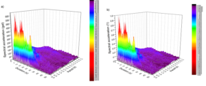
Based on the above definition, the time-frequency response spectrum of the M7.1 earthquake on May 18, 1940 in the EW direction of El Centro in Imperial Valley, USA was plotted (Figure 1a). Since the time-frequency response peaks of seismic waves are all different, the coordinate axis ratios are very different too. To make the result comparable, the normalization method is adopted in this paper. A special normalization method is:Relying on this conclusion, a normalization method concerning timefrequency response spectrum is presented. Normalized time-frequency response spectra of the El Centro earthquake wave from east to west are shown in Figure ref f1 b. It should be mentioned here that the spectral shape of the time-frequency response spectrum is almost the same as that of the normalized time-frequency response spectrum, but the number of Z-axis endpoints of the normalized time-frequency response spectrum is one.

IV. Example of time-frequency response spectrum analysis

IV.A. Typical seismic wave

To plot the contour plots of the normalized time-frequency response spectra of each seismic wave, the normalized time-frequency response spectra of the 1940 Imperial Valley Earthquake (El Centro EW seismic wave), the 1995 Kobe Earthquake (Kobe EW seismic wave), and the 2008 Wenchuan Earthquake in China (Wenchuan EW seismic wave) were calculated and presented in the form of Figures 2-3. This contour map can clearly reflect the time-frequency response characteristics of different types of seismic waves. Because the Wenchuan seismic wave has a long duration, the part of 20 s-90 s, where the amplitude of EW ground motion is larger, was selected as the effective ground motion duration.

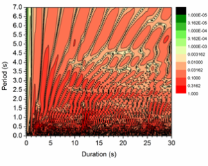
It can be seen from Figure 2 that the time-frequency response spectrum of the El Centro EW seismic wave has about three peak regions closely arranged along the duration direction. In contrast, the peak distribution along the natural vibration period direction is narrower, and the base distribution along the natural vibration period is wider. As can be seen from Figure 2b, the El Centro EW seismic wave lasts for 53.0 s, and its time-frequency response spectrum spreads over a big area in the region of the second-level peak (the region with the darker red color). This spectrum essentially covers the zone with 2.5 s-7.0 s duration and 0.0 s-4.5 s natural vibration period as well as the zone with 7.0 s-29.0 s duration and 0.0 s-2.9 s natural vibration period. However, it is small in area by the first-level peak region of the time-frequency response spectrum (the part covered with dark red color), including just the area with 1.0 s-15.0 s duration and 0.0 s-0.8 s natural vibration period. It is anticipated that structures with a natural vibration period of 0.0 s-0.8 s will enter plastic deformation at the region of the first-level ridge when subjected to the input of moderate-intensity ground motion. Then, the natural vibration period increases while further damage accumulates with second and lower-level ridges. For the structure having a natural vibration period of more than 0.8 s, it only experiences second and lower-level ridges. Even if the structure suffers minor damage, the cumulative damage will not appear in the subsequent small peak regions.

The time-frequency response spectrum in the direction of Wenchuan EW has an obvious temporal sequence, that is, there are three relatively independent spikes in the time domain. The height of these peaks is not fixed but gradually decreases with the increase of the duration. This variation is characterized by a gradual dissipation of the energy of the seismic wave with time. The bottom region of the wave peaks is smaller and the distribution is narrower in the intrinsic oscillation period at 0.0 s\(\mathrm{\sim}\)0.8 s. The wave peaks are characterized by a narrower distribution in the intrinsic oscillation period. As shown in Figure 3b, the spectral peak area of the Wenchuan EW-directed seismic wave can be divided into three zones: The area between the 8.0 s-16.0 s duration and 0.0 s-0.8 s natural vibration period; the area between the 29.0 s-38.0 s duration and 0.0 s-0.7 s natural vibration period; the area between 64.5 s-65.5 s duration and 0.0 s-0.3 s natural vibration period (the part with dark red color). Although the duration of the Wenchuan EW seismic wave is up to 70.0 s, its first-level ridge region is narrowly distributed in the time-frequency response spectrum between the natural vibration period of 0.0 s and 0.5 s, and its second-level ridge region is narrowly distributed in the natural vibration period of 0.0 s-0.8 s. When subjected to moderate-intensity ground motion inputs, structures with a natural vibration period of 0.0 s-0.5 s tend to enter plastic deformation and suffer cumulative damage. For structures with a natural vibration period of 0.5 s-0.8 s, minor damage may occur. For structures with natural vibration periods greater than 0.8 s, only third- or lower-level ridges will be encountered, and the potential for structural damage is very low.

IV.B. Ground motion with abundant low-frequency components

Ground shaking which is rich in low-frequency contents causes maximum damage to structures with a long self-oscillation period. For instance, a 7.7-magnitude earthquake that struck the middle area of the Sea of Japan in 1983 resulted in overflow and damage to the roof appurtenances of oil tanks in Niigata City, which is approximately 270 km from the epicenter, with a vibration period of about 10 s; A gigantic 8.1 magnitude earthquake in Mexico in 1985 destroyed high-rise buildings in Mexico City, about 400 kilometers from the center. Thus, the study of ground motion with abundant low-frequency components can help reduce the increasing seismic damage to high-rise and large-span structures.

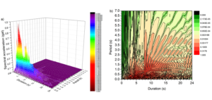
The 1999 Chi-Chi earthquake in Taiwan caused significant structural damage and a long-term natural shaking cycle. Figure 4 shows the time-frequency response spectrum and its contours for the TCU 115 stations. The time-frequency response spectrum in Figure 5a contains multiple peak regions. Compared with the peak region in Figure 5a, these peak regions are not distributed in a narrow band along the short natural vibration period direction but are sparsely distributed along the long natural vibration period direction. From Figure 5b, it can be seen that the first-level ridge region of the time-frequency response spectrum, i.e., the region in dark red color, covers basically the region of a long natural vibration period from 2.0 s to 6.5 s. The second-level ridge region (the part with darker red color) covers the whole natural vibration period axis of Figure 5b (0.0 s-7.0 s), showing a tendency to develop in the direction of more than 7.0 s. When subjected to moderate intensity ground motion inputs, structures with long natural vibration periods are likely to enter plastic deformation in the region of the first-level ridge. Even though the structure doesn’t collapse, it is sure to suffer damage owing to an increase in natural vibration period from the ridge action at the second level. The result above tells why a ground motion abundant in low-frequency components more readily causes damage to a structure having a long period of vibration.

IV.C. Pulse-like ground motion

This project proposes to select observations from the newly discovered Pico Canyon station (N46 W) from the 1994 Northridge earthquake and compare them with the N35 W station (N35 W) from the same earthquake. The normalized time-frequency response spectra and contour maps of the two seismic waves were separately plotted (Figures 5-6).

It can be seen from Figure 5a that the time-frequency response spectrum of Northridge pulse-like ground motion has only one peak and appears as a “cone”. The area of the “cone” bottom is very large and covers most of the duration-natural vibration period plane. In contrast, the time-frequency response spectrum of Northridge non-pulse-like ground motion has approximately two peaks, but the area covered by the bottom of the peak is smaller, with only a small area near the origin of the duration-natural vibration period plane (Figure 6a).

The first-level ridge of the time-frequency response spectrum of the Northridge pulse-like earthquake (the part with dark red color) covers a large area, roughly including the area with a duration of 5.0 s-12.0 s and a natural vibration period of 0.0 s-3.4 s. The second-level ridge region (the portion with darker red color) also extends to the zone of 4.0 s-20.0 s duration and natural vibration period of 0.0 s-5.0 s as well, shown in Figure 5b. Under the ground motion of moderate intensity, the structural response in all ranges of the natural vibration period before 4.0 s duration is small. After 4.0 s, the structure with the natural vibration period between 0 s-3.4 s will be continuously acted upon by the first-level ridge of the time-frequency response spectrum, with a high possibility of plastic deformation and collapse damage caused by moderate ground motion inputs. Even though the collapse does not occur at the first-level ridge, it still occurs because of the plastic deformation of the structure, increase in natural vibration period, and successive impact of the second-level ridges in the duration direction. Regarding the time-frequency response spectrum of the Northridge non-pulse-like ground motion in Figure 6b, the first-level ridge area of it only occurs below 0.5 s of the natural vibration period. Therefore structures whose natural vibration periods are greater than 0.5 s incur little damage from this input.

Therefore, compared with non-pulse-like ground motion, pulse-like ground motion is more likely to cause collapse damage to structures, especially to structures with long natural vibration periods. This result is consistent with the study of Bertero et al. [20].

V. Conclusion

In this paper, the commonly used seismic wave analysis methods (reaction spectrum, Fourier spectrum, power spectrum, wavelet analysis, HHT) are reviewed, with emphasis on the reaction spectrum analysis method.

Ground shaking time course cannot reflect the changes in ground shaking time course. The elastic-plastic time-range analysis method is complex and time-consuming, and its accuracy depends on the fine dissection of finite elements, the inherent intrinsic relationship of the material, and the selection of the ground-shaking waveform. On this basis, the seismic wave time-frequency response spectrum is established. The time-frequency response spectrum is a spatial spectrum that synthesizes the amplitude, spectrum and duration of ground shaking, and can reflect the relationship between the amplitude and duration of ground shaking. In order to facilitate the calculation, its maximum response value is used to classify the ground vibration wave spectrum. On this basis, a new normalized time-frequency analysis method is proposed and analyzed.

The normalized time-frequency response spectra of four representative seismograms, namely El Centro EW seismogram, Kobe EW seismogram, and Wenchuan EW seismogram, are comparatively studied in this section to reveal their relation to seismic activity. It was observed that there were noticeable differences in the magnitude distribution of each seismogram in both time and frequency domains.

Therefore, the “suitable” seismic data in the seismic design should be selected according to different tectonic types; otherwise, the results will be less credible. Based on this, the normalized time-frequency response spectrum (NTRS) method is applied to study the impulsive ground motion and ground motion with rich low-frequency components. This method can reflect the damage mechanism of the structure under seismic action more intuitively. However, the analysis in this paper is qualitative in nature and detailed calculations and verification of the seismic performance of the structure are yet to be carried out. The previous work of this group is summarized.

Acknowledgments

The support of Frontier Research Team of Kunming University 2023 is gratefully acknowledged. The authors also acknowledge the financial support from the Applied Basic Research Foundation of Yunnan Province (Grant No. 202101AT070144, Grant No. 202401CF070004) and Yunnan Provincial Department of Education Science Research Fund Projects (Grant No. 2023J0823). The authors also acknowledge the support of Kunming University Science and Technology Innovation Team 2020.