
Housing prices have been a longstanding focus in academic and practice research. Non-arm’s length transactions affect the real estate market since they are governed by so-called special relationships. These transactions include those between family and friends and those associated with urgent buying and selling, debt obligations or offsetting, and government agencies. Therefore, the sales prices in non-arm’s length transactions differ from those in normal or arm’s length transactions. To date, a few studies in Taiwan has examined the extent to which non-arm’s length transactions affect housing prices [1]. In the real estate market, the price differences between non-arm’s length and arm’s length transactions are often determined through the participants’ subjective experiences, which are not scientifically supported or verified objectively.
Price is established based on human factors, as our needs and wishes often play an important role in sales prices. Social capital refers to the benefits derived from human connections. Sociologists first conceptualized it to explain that the resources embedded in interpersonal relationships between communities, friends, colleagues, and family members can be used to help create personal social capital and wealth [2]. The social capital concept is salient in economics, management, politics, and behavioral theory. The existing research has primarily examined social capital in the context of real estate management, knowledge sharing, and internet use [3], [4], as well as farmland transactions [5]–[7]. Only a few studies have applied social capital pathways in the housing market [1], [8]. Social capital theory can be used to analyze the perceived price differences between arm’s length and non-arm’s length transactions, which often entail the personal relationships between buyers and sellers.
Previous empirical studies on the price differences between two housing types, such as foreclosed and non-foreclosed homes or houses located within or beyond elite school districts, have used the hedonic price approach for analysis. In these studies, the comparisons are based on different dummy variables. However, this approach neglects the effects of selection bias or data homogeneity, so the estimation results do not accurately reflect the price differences between the two groups [9], [10]. Most data in social science research are observational, such as real estate market prices, and are not derived through randomized experiments. Researchers often have no control over the mechanisms of participant allocation (to the treatment or control group) which are governed by other mechanisms or the participants’ self-selection [11]. Neglecting the problem of self-selection can result in endogenous bias and inconsistent estimations. This type of bias is known as selection bias [12]. Lee et al. [1] failed to address selection bias in their data, assigning transactions involving urgent buying/selling and government agencies to the same category and not considering the price discount differences between them. In this study, we matched the data using Rosenbaum & Rubin [13] propensity score matching (PSM) method, which addresses selection bias and omitted variable bias in large samples and further identifies the factors affecting housing prices [9], [14]. Social capital was represented by seven types of non-arm’s length transactions in the treatment group: with first-degree relatives, with second-degree relatives, with third-degree relatives, with friends, debt obligations, urgent buying/selling, and with government agencies. The control group consisted of arm’s length transactions. The transactions were matched with those in the other group to identify homogenous transactions and examine the price differences solely due to special relationships.
The literature review covers social capital and the application of PSM in real estate research. Robison et al. [6] defined social capital as a person’s or group’s obligations or sympathy toward another person or group. To date, most research on price differences in real estate products arising from buyer-seller or personal relationships has focused on farmland transactions [5], [7], [15]–[18]. Few studies have applied social capital in housing price research [1], [8].
Siles et al. [7] studied farmland transactions in Illinois, Michigan, and Nebraska and demonstrated the effects of specific interpersonal relationships on sales prices. The offered prices differed significantly between strangers, neighbors, influential people, and relatives. The highest prices were offered to unfriendly neighbors, while the lowest prices were offered to friendly relatives, thus supporting the social capital hypothesis. Perry & Robison [17] explored the role of personal relationships in farmland transactions in Linn County, Oregon. Family relationships consisted of parent and child, grandparents and grandchildren, siblings, and other family members; non-familial relationships consisted of strangers, neighbors, and acquaintances. Their results showed that parent-child relationships had the most significant effects on farmland prices, with reductions from 31% to 38%. The price reductions in transactions between neighbors were 11% to 23%, slightly higher than those between other family members, which were 7% to 19%. The price reductions in transactions with former tenants were 9% to 12%, while those in transactions with acquaintances were 0% to 10%. Kostov, Patton, & McErlean [16] used nonparametric neural networks in their analysis. They found that buyer characteristics and personal relationships influenced the sales terms in the farmland market and validated the social capital assumption. Pitts [5] examined whether farmland leasing in Kansas was affected by social capital, revealing that a longer lease term and good tenant-landlord relations resulted in a lower lease rate, thus bolstering the important influence of social capital on farmland leases in Kansas. Lee et al. [1] included personal relationship-related variables in their hedonic price function and used personal relationships to represent the effects of social capital. Their sample consisted of registered housing data in Taipei City from January 1, 2012, to December 31, 2018. Their empirical results showed that housing sales involving debt obligations and urgent buying/selling were 22.6% lower than those in arm’s length transactions, while transactions with government agencies were 48.9% lower. Transactions between first-, second-, and third-degree relatives were 57.3%, 53.1%, and 50.3% lower than those in arm’s length transactions, with the premiums decreasing with an increasing degree of consanguinity. Transactions with friends were 28.0% lower than those in arm’s length transactions. Pilatin [8] applied panel data regression analysis to examine the effects of social capital on the housing price index in Turkey. The results revealed that social capital significantly and negatively influenced the panel data regression analysis.
Most of the literature has used regression analysis to investigate the influence of events on housing prices. When used in observational studies, regression analysis often results in endogeneity or self-selection bias, thus reducing the accuracy of the estimations and causal inference [19] because important variables cannot be controlled, and important independent variables are omitted. Moreover, endogeneity or self-selection bias emerges when the observed events do not occur randomly, resulting in inaccurate findings. Rosenbaum & Rubin [13] proposed PSM to resolve to increase the data homogeneity between the treatment and control groups and resolve self-selection bias. Many researchers have endorsed PSM as a suitable preprocessing technique for reducing noise from a mix of characteristics [20]–[22]. Wall [22] argued that PSM is the most popular matching technique as it can convert a set of covariates into a propensity score. Two sets of housing attributes are more similar when their propensity scores are closer, minimizing the potential omitted variable bias. In this study, we matched the treatment and control groups through PSM. Despite being widely used in international studies, there is significant room for developing the application of PSM in real estate research in Taiwan.
Regarding applying PSM in real estate research, in terms of real estate policy evaluation, Andersen & Nielsen [23] used PSM to ensure that the sample variables were homogenous. Because Danish regulations stipulate that beneficiaries must sell their inheritance within 12 months, forced house sale prices are lower than comparable houses in the market, and greater discounts are offered as the deadline approaches. Locke et al. [24] used PSM to investigate the influence of land use zoning regulations on the quantity of housing units. Comparisons made at the same or similar conditions can yield more accurate estimations. Their results revealed that implementing zoning regulations increased the number of housing units in high-income townships but decreased it in low-income townships. Nanda & Ross [25] investigated the influence of sellers’ disclosure of their property’s condition on real estate value by combining PSM with a traditional event study approach. Their results showed that property condition disclosure laws resolved the information asymmetry in housing sales so that the buyer was more confident in the quality of the house they bought. This observation became more prominent after PSM. Liu & Lynch [26] applied PSM to resolve sample selection bias. Homogenizing the attributes of the treatment and control groups was helpful for investigating the impacts of land preservation programs on farmland loss. Their findings highlighted the practical benefits of these programs, leading them to conclude that they reduced the rate of farmland loss. Walls et al. [27] also applied PSM to address sample selection bias and estimated that verified energy-saving homes were more expensive than unverified homes. They underscored the importance of PSM as it increased the accuracy of estimating the spillover effects of energy-saving homes. Lee et al. [28] applied PSM to minimize estimation bias. They incorporated the difference-in-differences (DID) approach and spatial quantile regression in their model to analyze the spillover effects of urban renewal at different stages on nearby housing prices. Their results highlighted that the spillover effects were overstated in previous studies, and PSM increased the accuracy of their results. Lee et al. [29] applied PSM to address data homogeneity. They integrated DID and a two-stage spatial quantile regression model to investigate how housing prices are affected by the announcement of areas at risk of soil liquefaction. Their results indicated that the risk of soil liquefaction had the greatest effect on low housing prices.
To reduce bias in observational research, Wen [30] emphasized that matching, stratification, and adjustment confounders should be used appropriately to control the confounding effects. Various potential confounders exist in the real estate domain, such as house age, floor area, and building material. Developed by Rosenbaum & Rubin [31], PSM can be used to control the confounding effects. One advantage of PSM is that estimating a single propensity score is sufficient for comparison and matching. PSM is relatively simpler, more convenient, and more powerful than other variable matching methods [32]. In social sciences, PSM is often used to examine the effects of a policy change on individuals. Researchers propose a causal assumption and analyze the causal effects of the policy change on individuals. The key to correct causal inferences lies in group allocation in comparative research. Grouping based on the internal factors (endogeneity) of causality can result in identifying the average causal effect [11]. PSM is a counterfactual model of causality that resolves the identification problem [33]. In PSM, the sample is divided into treatment and control groups. Matching aims to control the covariates so that both groups are similar or consistent except for the treatment. In practice, logistic regression is used to calculate the propensity score of each sample based on the information provided by the matching variables. The samples with the closest propensity scores derived through different matching methods in both groups are matched. The derived estimates differ according to the matching method [34]. Common matching methods include nearest neighbor matching (NNM), radius matching, stratification matching, and kernel matching [35]. Lastly, the average treatment effect on the treated (ATT) is calculated through counterfactual inference.
This study used the NNM approach, which is a simple nonparametric categorization approach [36]. In PSM, a caliper is set, and the matching sample is identified as the number of nearest neighbors (designated as k, a positive and complete integer that is often odd) within the caliper widths. The accuracy of the results depends on the quality of the sample database. While the sample size obtained through NNM is small, the bias is low because the samples are nearly identical. Several tests are required after matching to ensure the quality of the matching process. The common support is identified to check for matching variables with the same scores and to ensure that they are equally likely to be assigned to the treatment or control group. If a piece of data is likely to be assigned to one group only, it will be excluded from the common support and analysis [37]. Balance represents the similarity in the distribution of control variables in the two groups. A common problem in PSM is whether the propensity-scored variables can balance the initial differences between the treatment and control groups. Rosenbaum & Rubin [31] suggested that propensity scores have balancing functions. A pair of matched samples are obtained after matching and must undergo balance testing so that the control variables have a similar likelihood of being assigned to either group. After determining the balanced sample, the uncertainty or the risk of hidden bias arising from estimation errors must be evaluated (i.e., the aforementioned likelihood is influenced not only by the observable variables but also by the non-observable variables). Therefore, sensitive analysis is required to treat the potential risks to the ATT and the interference caused by selective bias [37]. This study applied [38] bounding approaches to perform a sensitivity analysis of the variables and identify the presence of severe bias caused by non-observable variables.
In Rosenbaum’s bounding approach, the critical value Γ is derived from the absolute estimate and represents the measured degree of unobserved bias. Duyvendack & Palmer-Jones [39] suggested that the matching estimates may be confounded by unobservable variables when Γ is very small (typically <2) and the generated confidence interval includes 0.
The dependent variable in this study was the logarithm of the total housing price. The independent variables included housing structure attributes, neighborhood attributes, administrative district, non-arm’s length transactions, and time trends. Based on the model settings in the studies by [40]–[42] seven dummy variables related to non-arm’s length transactions were established: transactions with first-degree relatives, second-degree relatives, third-degree relatives, friends, government agencies, and those involving debt obligations and urgent buying/selling. Houses in arm’s length transactions served as the baseline. The settings and descriptions of the variables are presented in Table 1, and the model settings are shown in Eq. (1):
\[\begin{aligned} \label{GrindEQ__1_} InP_i=&{\alpha }_1+{\alpha }_2AREA+{\alpha }_3AGE+{\alpha }_4AGES+{\alpha }_5ROOM+{\alpha }_6LIVROOM+{\alpha }_7BATH\notag\\&+{\alpha }_8FLOOR1+{\alpha }_9FLOOR4+{\alpha }_{10}TYPE1+{\alpha }_{11}TYPE2+{\alpha }_{12}DISTMRT\notag\\&+{\alpha }_{13}DISTHIGHSCH+{\alpha }_{14}DISTMIDSCH+{\alpha }_{15}DISTELESCH+{\alpha }_{16}DISTCBD\notag\\&+{\alpha }_{17}DISTTRAIN+\sum^{23}_{j=1}{{\gamma }_j{ADMINIST}_j}+\sum^7_{k=1}{{\beta }_k}{RELATED}_k+\sum^7_{l=1}{{\theta }_l}{TREND}_l+{\varepsilon }_i , \end{aligned}\tag{1}\]
| Variable | Description | Expected symbol |
|---|---|---|
| Dependent variable | + | |
| 1-2 Total sales price (lnPi) | The logarithm of the registered real estate total sales price. Unit in NT$10,000. | |
| 1-2 Independent variables | ||
| 1-2 Floor area (AREA) | A continuous variable. Defined as the registered building transfer area. Unit in ping (3.31 m2). | |
| House age (AGE) | A continuous variable. Defined as the difference between the construction completion date and the sales date. Unit in years. | − |
| House age squared (AGES) | A continuous variable. Unit in years. | + |
| Number of rooms (ROOM) | A continuous variable representing the number of rooms in a house. | + |
| Number of living rooms (LIVROOM) | A continuous variable representing the number of living rooms in a house. | + |
| Number of bathrooms (BATH) | A continuous variable representing the number of bathrooms in a house. | + |
| Floor level (FLOOR) | A dummy variable. For FLOOR1, houses on the first floor are assigned 1, while houses on other floors are assigned 0. For FLOOR4, houses on the fourth floor are assigned 1, while houses on other floors are assigned 0. | +/ _ |
| Housing type (TYPE) | A dummy variable. Housing types consist of apartment buildings, condominiums, and luxury condos, with condominiums serving as the baseline. For TYPE1, houses in apartment buildings are assigned 1, while other houses are assigned 0. For TYPE2, houses in luxury condos are assigned 1, while other houses are assigned 0. | + |
| Distance to the nearest MRT station (DISTMRT) | A continuous variable representing the distance from a house to the nearest MRT station. Unit in meters. | _ |
| Distance to the nearest senior high school (DISTHIGHSCH) | A continuous variable representing the distance from a house to the nearest senior high school. Unit in meters. | _ |
| Distance to the nearest junior high school (DISTMIDSCH) | A continuous variable representing the distance from a house to the nearest junior high school. Unit in meters. | _ |
| Distance to the nearest elementary school (DISTELESCH) | A continuous variable representing the distance from a house to the nearest elementary school. Unit in meters. | _ |
| Distance to the city center (DISTCBD) | A continuous variable representing the distance from a house to the city center. Unit in meters. The center of Taipei City is the Zhongxiao Fuxing MRT Station [45], and the center of New Taipei City is the Banqiao Station. | _ |
| Distance to the nearest railway station (DISTTRAIN) | A continuous variable representing the distance from a house to the nearest railway station. Unit in meters. | _ |
| Administrative district (ADMINIST) | Twenty-three dummy variables are established, one for each of the 12 administrative districts in Taipei City and 12 selected districts in New Taipei City. Wanhua District serves as the baseline as it has lower housing prices. | +/− |
| RELATED | Seven dummy variables are established (\(RELATED_{k} ,{\rm ; }k=1\sim 7.\)), with arm’s length transactions serving as the baseline. The types of non-arm’s length transactions were those between first-, second-, and third-degree relatives; those associated with debt obligations or offsetting; those involving urgent buying/selling; those with government agencies; and those with friends. | _ |
| TREND | Seven dummy variables are established for the data period spanning January 1, 2012, to December 31, 2019, with 2012 serving as the baseline. These variables capture changes in the trends of arm’s length transaction prices in the real estate market. | +/− |
where \( \ln P_i \) is the logarithm of the sales price of the i-th house, \( \alpha_1 \) is the intercept, \( \alpha_2 \)–\( \alpha_{11} \) are the coefficients of the housing structure attribute variables, \( \alpha_{12} \)–\( \alpha_{17} \) are the coefficients of the neighborhood attribute variables, \( \gamma_j \) is the coefficient of the attribute variable relating to the 23 administrative districts across the study area, \( \beta_k \) is the coefficient of the variable relating to the seven types of social capital (non-arm’s length transactions), \( \theta_l \) is the coefficient of the variable relating to the seven time points, and \( \varepsilon_i \) is the error term for a normal distribution.
Designating the total sales price as a dependent variable can better reflect the overall housing price and enable more efficient observation of complete data during estimation. Previous studies have also used the logarithm of the total housing price for estimation [43], [44]. The dependent variable in this study was the logarithm of the total sales price \( (\ln P_i) \).
Based on the data registered in the Ministry of the Interior’s real estate actual price registration system, we categorized variables affecting housing price into four types: housing structure attributes (floor area, house age, floor level, housing type, and number of rooms, living rooms, and bathrooms), neighborhood attributes (distance to the nearest mass rapid transit [MRT] station, railway station, senior high school, junior high school, elementary school, and city center), administrative district attributes (housing location), and type of transaction (arm’s length and non-arm’s length). The variable types are specified in Table 1.
Several important variables are elucidated as follows: The type of transaction included arm’s length and non-arm’s length transactions. Non-arm’s length transactions include those between first-, second-, and third-degree relatives; those involving debt obligations or offsetting; those associated with urgent buying/selling; those with government agencies; and those with friends. Seven dummy variables were established, each representing a type of non-arm’s length transaction, with arm’s length transactions serving as the baseline. The coefficients are expected to be significantly lower for the seven types of non-arm’s length transactions than for normal arm’s length transactions.
TREND is the dummy variable of time and captures the changes in the trends of arm’s length transaction prices in the real estate market. The data spanned January 1, 2012, to December 31, 2019. Seven dummy variables were established, each representing a year during this period, with 2012 serving as the baseline.
In July 2012, Taiwan announced the implementation of a real estate actual price registration system to increase the transparency of sales information. Most people rely on the system to query previous sales prices and relevant information. Non-arm’s length transactions, such as those between employees who are relatives or friends, those involving urgent buying/selling or debt obligations/offsetting, and those with government agencies, are also indicated alongside the sales prices in the system. These sales prices may deviate from current market prices in arm’s length transactions or be heavily discounted.
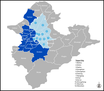
This study sourced the housing transaction data from the Ministry of the Interior’s real estate actual price registration system (Ministry of the Interior, 2018). The housing transaction data spanned from January 1, 2012, to December 31, 2019, and covered the cities of Taipei and New Taipei. In the latter, 12 administrative districts that are as developed as all of the 12 administrative districts in the former were selected: Banqiao, Xinzhuang, Zhonghe, Yonghe, Sanchong, Shulin, Xindian, Taishan, Wugu, Luzhou, Tucheng, and Tamsui (Figure 1). The main housing types were apartment buildings, luxury condos, and condominiums. The sample consisted of single non-arm’s length transactions. Data related to duplicate non-arm’s length transactions based on the remarks column; houses with extreme prices; houses with more than five rooms, living rooms, or bathrooms; and houses older than 60 years were excluded. The dataset comprised 83,604 transactions: 24,451 in Taipei City and 59,153 in New Taipei City.
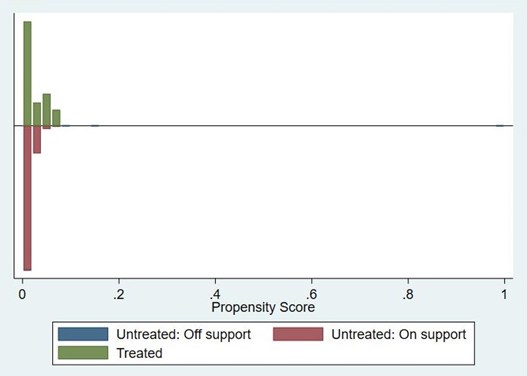
As shown in Figure 2, all transactions in the treatment group are within the common support of the distributions of propensity scores in each group (on-support), while a few in the control group are outside the common support (off-support). Of the 83,604 transactions before matching, the 50 off-support transactions were removed, leaving 83,554 for analysis and matching.
The balance in the variables should be assessed after PSM. Garrido et al. [12] suggested that t-tests can be used to assess the initial balance. As shown in Table 2, among the eight continuous variables, AGE, AREA, DISTCBD, DISTELEESCH, and DISTHIGHSCH were significant before matching but were not significant after matching, meaning that the initial balance tests were good.
| Independent variables |
Sample | Bias(%) | %Reduction in |bias| |
t-test | ||
|---|---|---|---|---|---|---|
| t | p | |||||
| ROOM | Unmatched Matched |
-2.5 -2.9 |
-13.0 | -0.80 -0.65 |
0.421 0.519 |
|
| LIVROOM | Unmatched | 2.8 | 0.90 | 0.369 | ||
| Matched | -2.4 | 12.3 | -0.58 | 0.562 | ||
| BATH | Unmatched | 2.4 | 0.79 | 0.432 | ||
| Matched | -6.5 | -168.8 | -1.49 | 0.136 | ||
| AGE | Unmatched | 26.6 | -9.86 | 0.001*** | ||
| Matched | 6.0 | 77.6 | 1.34 | 0.179 | ||
| AREA | Unmatched | 21.4 | 7.77 | 0.001*** | ||
| Matched | -1.7 | 92.2 | -0.33 | 0.741 | ||
| DISTCBD | Unmatched | -48.2 | -13.98 | 0.001*** | ||
| Matched | -4.1 | 91.6 | -1.07 | 0.283 | ||
| DISTELESCH | Unmatched Matched |
-33.7 -2.1 |
93.8 | -9.99 -0.53 |
0.001*** 0.595 |
|
| DISTHIGHSCH | Unmatched Matched |
-17.0 -5.4 |
68.5 | -4.77 -1.39 |
0.001*** 0.165 |
|
| Note: Unmatched represents variables before matching, and matched represents variables after matching; *, **, and *** represent a significance level of 10%, 5%, and 1%, respectively. |
||||||
| Independent variables | Sample | Chi-squared | p-value |
|---|---|---|---|
| FLOOR1 | |||
| Unmatched Matched |
3.2119 0.0882 |
0.073*0.766 | |
| FLOOR4 | Unmatched | 7.4926 | 0.006*** |
| Matched | 6.1011 | 0.014** | |
| TYPE1 | Unmatched | 94.4576 | 0.001*** |
| Matched | 43.4544 | 0.001*** | |
| TYPE2 | Unmatched | 33.2726 | 0.001*** |
| Matched | 14.67 | 0.001*** | |
| DISTMRT500 | Unmatched | 0.2255 | 0.635 |
| Matched | 0.0756 | 0.783 | |
| Note: *, **, and *** represent a significance level of 10%, 5%, and 1%, respectively. | |||
However, Garrido et al. [12] also noted that assessing the balance after matching solely through t-tests is inadequate since the smaller sample size after matching can reduce the statistical power of such tests, resulting in them no longer being significant, and thus the matching results are unbalanced [20], [46]. Studies [13], [47] showed that besides using standardized differences in balance diagnostics, two independent sample t-tests can be used before matching to assess the balance of continuous variables. If the t-tests indicate that the sample is balanced, then the sample should be double-checked using other balance tests to ensure accurate results. The chi-square test results of the categorical variables are shown in Table 3.
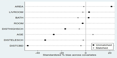
Rosenbaum & Rubin [13] conceptualized standardized bias as the difference in the means in units of pooled standard deviation [48]. This approach differs from t-tests and other hypothesized statistical tests as it is unaffected by the sample size. Therefore, it can be used to compare the balance in the measurement variables between the treatment and control groups [46]. This approach calculates the percentage variation in the standardized bias of an attribute variable between two samples. A positive and higher percentage indicates that an attribute variable has low variation within two samples, and, therefore, the matching is more efficient [9]. Table 2 and Figure 3 show the percentage variation in the standardized bias of all variables: LIVROOM = 12.3%, AGE = 77.6%, AREA = 92.2%, DISTCBD = 91.6%, DISTELEESCH = 93.8%, and DISTHIGHSCH = 68.5%. While the percentage variations in the standardized bias of ROOM and BATH were negative, the standardized bias after PSM was only –2.9% and –6.5%, respectively, without any significant bias. Moreover, the mean standardized bias decreased from 19.3% \(( [2.5 + 2.8 + 2.4 + 26.6 + 21.4 + 48.2 + 33.7 + 17.0] / 8 )\) to 3.9% \(( [2.9 + 2.4 + 6.5 + 6.0 + 1.7 + 4.1 + 2.1 + 5.4] / 8 )\), showing that PSM effectively reduced the variances of the variables.
Lastly, the sensitivity analysis results are shown in Table 4. As the critical value Γ gradually increased in 0.2 intervals to 2, the generated confidence intervals did not include 0, indicating that the estimated ATT was not confounded by non-observable variables, and the inference process was efficient.
| Γ | Hodges–Lehmann point estimates | 95% confidence interval | ||
|---|---|---|---|---|
| 2-5 | maximum | minimum | maximum | minimum |
| 1.00 | -6,000,000 | -6,000,000 | -6,500,000 | -5,400,000 |
| 1.20 | -6,700,000 | -5,200,000 | -7,400,000 | -4,600,000 |
| 1.40 | -7,400,000 | -4,600,000 | -8,100,000 | -4,000,000 |
| 1.60 | -8,000,000 | -4,000,000 | -8,700,000 | -3,400,000 |
| 1.80 | -8,600,000 | -3,500,000 | -9,300,000 | -2,900,000 |
| 2.00 | -9,100,000 | -3,100,000 | -9,800,000 | -2,400,000 |
Table 5 shows the descriptive statistics of the matched transactions. The mean housing price was NT$12.3 million, the mean number of rooms was 2.68, the mean number of living rooms was 1.74, the mean number of bathrooms was 1.51, the mean floor area was 31.60 ping, the mean house age was 21.58 years, the mean distance to the nearest MRT station was 785.95 meters, the mean distance to the nearest railway station was 3,780.21 meters, the mean distance to the nearest senior high school was 804.41 meters, the mean distance to the nearest junior high school was 645.52 meters, the mean distance to the nearest elementary school was 410.64 meters, the mean distance to the city center was 5,040.68 meters. Most transactions related to apartment buildings (43.99%), followed by condominiums (40.49%) and luxury condos (15.52%). First-floor houses accounted for 6.21% of transactions, fourth-floor houses accounted for 13.33%, and houses on other floors accounted for 80.47%. Arm’s length transactions accounted for 68.79% of all transactions, and non-arm’s length transactions accounted for 31.21%: those related to urgent buying/selling accounted for 1.22%, those related to debt obligations or offsetting accounted for 5.67%, those with government agencies accounted for 13.30%, those involving first-degree relatives accounted for 0.91%, those involving second-degree relatives accounted for 7.26%, those involving third-degree relatives accounted for 1.45%, and those involving friends accounted for 1.40%. The descriptive statistics of the treatment and control groups are shown in Table 6.
| All transactions (N=3,512) | Mean | Standard deviation (SD) | Minimum | Maximum |
|---|---|---|---|---|
| PRICE (in units of NT$10,000) | 1,230 | 1,100 | 100 | 31,000 |
| Number of rooms (ROOM) | 2.68 | 0.75 | 1 | 5 |
| Number of living rooms (LIVROOM) | 1.74 | 0.46 | 1 | 5 |
| Number of bathrooms (BATH) | 1.51 | 0.55 | 1 | 5 |
| Floor area (AREA) | 31.60 | 13.39 | 15.05 | 288.18 |
| House age (AGE) | 21.58 | 14.67 | 0.1 | 52.2 |
| Distance to the nearest MRT station (DISTMRT) | 785.95 | 697.95 | 8.06 | 7,264.63 |
| Distance to the nearest senior high school (DISTHIGHSCH) | 804.41 | 544.30 | 15.62 | 5,166.15 |
| Distance to the nearest junior high school (DISTMIDSCH) | 645.52 | 399.81 | 27.90 | 5,603.91 |
| Distance to the nearest elementary school (DISTELESCH) | 410.64 | 244.09 | 19.48 | 1,783.31 |
| Distance to the city center (DISTCBD) | 5,040.68 | 3,306.59 | 114.42 | 24,296.09 |
| Distance to the nearest railway station (DISTTRAIN) | 3,780.21 | 3,133.21 | 195.91 | 21,508.78 |
| Frequency | Percentage | Cumulative percentage | ||
| Housing type (TYPE) | ||||
| Apartment buildings | 1,545 | 43.99% | 43.99% | |
| Luxury condos | 545 | 15.52% | 59.51% | |
| Condominiums | 1,422 | 40.49% | 100.00% | |
| Floor level (FLOOR) | ||||
| First floor | 218 | 6.20% | 6.20% | |
| Fourth floor | 468 | 13.33% | 19.53% | |
| Other floors | 2,826 | 80.47% | 100.00% | |
| Type of transaction | ||||
| Non-arm’s length transactions | ||||
| Urgent buying/selling | 43 | 1.22% | 1.22% | |
| Debt obligations or debt offsetting | 199 | 5.67% | 6.89% | |
| Government agencies | 467 | 13.30% | 20.19% | |
| First-degree relatives | 32 | 0.91% | 21.10% | |
| Second-degree relatives | 255 | 7.26% | 28.36% | |
| Third-degree relatives | 51 | 1.45% | 29.81% | |
| Friends | 49 | 1.40% | 31.21% | |
| Arm’s length transactions | 2,416 | 68.79% | 100.00% | |
| Control group (N=2,416) | Treatment group (N=1,096) | |||||||
|---|---|---|---|---|---|---|---|---|
| Mean | SD | Min. | Max. | Mean | SD | Min. | Max. | |
| PRICE | 1,360 | 1,220 | 200 | 31,000 | 927 | 692 | 100 | 10,500 |
| ROOM | 2.68 | 0.77 | 1 | 5 | 2.66 | 0.69 | 1 | 5 |
| LIVROOM | 1.74 | 0.46 | 1 | 5 | 1.75 | 0.46 | 1 | 4 |
| BATH | 1.51 | 0.56 | 1 | 5 | 1.51 | 0.55 | 1 | 4 |
| AREA | 31.06 | 13.28 | 15.08 | 288.14 | 32.79 | 13.55 | 15.05 | 288.18 |
| AGE | 22.60 | 13.63 | 0.1 | 50.1 | 19.33 | 16.53 | 0.1 | 52.2 |
| DISTMRT | 854.20 | 762.83 | 8.06 | 7,264.63 | 635.49 | 495.60 | 22.32 | 7,019.21 |
| DISTHIGHSCH | 821.14 | 591.41 | 15.62 | 5,166.15 | 767.54 | 420.18 | 53.74 | 4,802.63 |
| DISTMIDSCH | 628.22 | 424.51 | 27.90 | 5,603.91 | 683.66 | 336.12 | 55.18 | 4,582.37 |
| DISTELESCH | 427.12 | 253.18 | 19.48 | 1,783.31 | 374.29 | 218.51 | 35.91 | 1,414.45 |
| DISTCBD | 5,336.31 | 3,400.0 | 114.42 | 24,296.09 | 4,388.98 | 2,990.67 | 492.09 | 23,366.83 |
| DISTTRAIN | 4,153.22 | 3,130.28 | 195.91 | 21,508.78 | 2,957.95 | 2,980.41 | 195.91 | 20,011.96 |
| Frequency | Percentage | Cumulative percentage | Frequency | Percentage | Cumulative percentage | |||
| Apartment buildings | 973 | 40.27% | 40.27% | 572 | 52.19% | 52.19% | ||
| Luxury condos | 413 | 17.10% | 57.37% | 132 | 12.04% | 64.23% | ||
| Condominiums | 1,030 | 42.63% | 100.00% | 392 | 35.77% | 100.00% | ||
| FLOOR | ||||||||
| First floor | 148 | 6.13% | 6.13% | 70 | 6.39% | 6.39% | ||
| Fourth floor | 345 | 14.28% | 20.41% | 123 | 11.22% | 17.61% | ||
| Other floors | 1,923 | 79.59% | 100.00% | 903 | 82.39% | 100.00% | ||
| Type of transaction | ||||||||
| Non-arm’s length transactions | ||||||||
| Urgent buying/selling | 43 | 3.92% | 3.92% | |||||
| Debt obligations or debt offsetting | 199 | 18.16% | 22.08% | |||||
| Government agencies | 467 | 42.61% | 64.69% | |||||
| First-degree relatives | 32 | 2.92% | 67.61% | |||||
| Second-degree relatives | 255 | 23.27% | 90.88% | |||||
| Third-degree relatives | 51 | 4.65% | 95.53% | |||||
| Friends | 49 | 4.47% | 100.00% | |||||
| Arm’s length transactions | 2,416 | 100.00% | 100.00% | |||||
The empirical results in Table 7 indicate that the F-statistic was 5697.93 and was significant at the 1% level before PSM, indicating that the regression model had a good model fit. The adjusted \( R^2 \) was 0.8025. Next, we checked for serious collinearity between the explanatory variables using the variance inflation factor (VIF). According to Kutner et al. [49], a VIF of <10 indicates the absence of serious collinearity between the explanatory variables, and the estimated coefficients are not seriously affected. The results showed that except for AGE and AGES, all variables had a VIF of <10. White [50] suggested that robust standard errors can be used to address the heteroscedasticity of the error terms. Therefore, we used robust standard errors to test and verify the assumptions.
| Unmatched | Matched | |||||
|---|---|---|---|---|---|---|
| Variable | Coef. | SE | p | Coef. | SE | p |
| Constant | 15.823 | 0.040 | 0.001*** | 15.943 | 0.061 | 0.001*** |
| Floor area | 0.016 | 0.005 | 0.001*** | 0.018 | 0.002 | 0.001*** |
| House age | −0.020 | 0.001 | 0.001*** | −0.020 | 0.002 | 0.001*** |
| House age squared | 0.001 | 0.001 | 0.001*** | 0.001 | 0.001 | 0.001*** |
| Number of rooms | 0.066 | 0.027 | 0.016** | 0.028 | 0.014 | 0.043** |
| Number of living rooms | 0.063 | 0.008 | 0.001*** | 0.006 | 0.015 | 0.679 |
| Number of bathrooms | 0.074 | 0.023 | 0.001*** | 0.102 | 0.019 | 0.001*** |
| First floor | 0.208 | 0.007 | 0.001*** | 0.195 | 0.028 | 0.001*** |
| Fourth floor | −0.031 | 0.002 | 0.001*** | −0.010 | 0.014 | 0.502 |
| Apartment building | 0.148 | 0.014 | 0.001*** | 0.191 | 0.023 | 0.001*** |
| Luxury condo | 0.109 | 0.014 | 0.001*** | 0.108 | 0.023 | 0.001*** |
| Distance to the nearest MRT station | −0.001 | 0.001 | 0.001*** | −0.001 | 0.001 | 0.001*** |
| Distance to the nearest senior high school | −0.001 | 0.001 | 0.001*** | 0.001 | 0.001 | 0.348 |
| Distance to the nearest junior high school | 0.001 | 0.001 | 0.430 | −0.001 | 0.001 | 0.001*** |
| Distance to the nearest elementary school | −0.001 | 0.001 | 0.001*** | −0.001 | 0.001 | 0.015** |
| Distance to the city center | −0.001 | 0.001 | 0.001*** | −0.001 | 0.001 | 0.001*** |
| Distance to the nearest railway station | 0.001 | 0.001 | 0.001*** | 0.001 | 0.001 | 0.001*** |
| Transactions with first-degree relatives | −0.766 | 0.091 | 0.001*** | −0.762 | 0.088 | 0.001*** |
| Transactions with second-degree relatives | −0.725 | 0.033 | 0.001*** | −0.722 | 0.033 | 0.001*** |
| Transactions with third-degree relatives | −0.645 | 0.086 | 0.001*** | −0.639 | 0.085 | 0.001*** |
| Debt obligations or debt offsetting | −0.094 | 0.033 | 0.004*** | −0.128 | 0.033 | 0.001*** |
| Transactions with government agencies | −0.792 | 0.025 | 0.001*** | −0.600 | 0.033 | 0.001*** |
| Urgent buying/selling | −0.216 | 0.045 | 0.001*** | −0.244 | 0.044 | 0.001*** |
| Transactions with friends | −0.262 | 0.048 | 0.001*** | −0.305 | 0.051 | 0.001*** |
| Fixed effects of time | yes | yes | yes | yes | ||
| Fixed effects of administrative district | yes | yes | yes | yes | ||
| F | 5697.93 | 180 | ||||
| R2 | 0.8026 | 0.7351 | ||||
| Adjusted R2 Prob > F Root MSE | 0.8025 0.001 0.233 | 0.7310 0.001 0.306 | ||||
After PSM, the regression model had an F-statistic of 180 and was significant at the 1% level, indicating that the model had a good model fit. The adjusted R 2 was 0.7310. The results showed that except for AGE, AGES, DISTCBD, DISTTRAIN, and ADMINIST22 (Tamsui District), all variables had a VIF of <10.
Regarding the differences in the regression model before and after PSM, the coefficients of the number of living rooms, fourth-floor houses, and distance to the nearest senior high school became significant after PSM. The coefficient difference was largest for the variable of transactions with government agencies, which decreased from −0.792 before matching to −0.600 after PSM.
Regarding the estimated results for housing structure attributes in the matched empirical results, the direction and estimated coefficients of all variables except for the number of living rooms and fourth-floor houses were significant and consistent with previous studies. Regarding the estimated results for neighborhood attributes, the direction and estimated coefficients of all variables were significant and consistent with previous studies, except for distance to the nearest railway station (positive) and distance to the nearest senior high school (positive and not significant).
The estimated coefficient of transactions involving debt obligations or offsetting was −0.128 and significant at the 1% level, indicating that the sales prices in these transactions were 12.0% (antilog-transformed value, same for all subsequent values in this section) lower than in arm’s length transactions. The estimated coefficient of transactions involving urgent buying/selling was −0.224 and significant at the 1% level, indicating that the sales prices in these transactions were 21.7% lower than in arm’s length transactions. The estimated coefficient of transactions with government agencies was −0.600 and significant at the 1% level, indicating that the sales prices in these transactions were 45.1% lower than in arm’s length transactions. The estimated coefficients of transactions with first-, second-, and third-degree relatives were −0.762, −0.722, and −0.639, respectively, and all were significant at the 1% level, indicating that the sales prices in these transactions were 53.3%, 51.4%, and 47.2% lower than in arm’s length transactions, respectively. The estimated coefficient of transactions with friends was −0.305 and significant at the 1% level, indicating that the sales prices in these transactions were 26.3% lower than in arm’s length transactions.
The results revealed that transactions involving debt obligations or offsetting and urgent buying/selling had lower sales prices than transactions with friends, highlighting the importance of personal relationships or social connections. In theory, these relationships are known as social capital. The value of personal relationships on transactions involving debt obligations or offsetting and urgent buying/selling is purely grounded in financial interests, costs, and time.
Transactions with government agencies were considerably cheaper than arm’s length transactions because the government aims to promote land use, reduce the management load, and gain more government revenue by selling real estate, preferably publicly-owned properties not intended for public use. These properties are often vacant, left empty, or occupied by others. To maximize the utilization of land resources, the government adopts measures such as allocation, leasing, selling small plots of land, selling leased land, selling projects, selling by tender, or outsourcing operations. For example, it is difficult to reacquire a plot of land occupied by a private legal building. Therefore, to minimize the cumbersome processes, the government often sells its properties at a self-designated discount to buyers in need; therefore, transactions with government agencies are often cheaper than arm’s length transactions.
In this study, the transactions with government agencies included public tendering by the Department of Rapid Transit Systems, Taipei City Government. These transactions often involve integrated residential buildings connected to MRT stations. To increase land use, the government jointly develops these buildings with construction firms and then sells them through public tender, similar to foreclosure sales. However, these houses are relatively cheaper than current market prices because there is little information available online, the tender schedule is not publicly announced, and there are no warranty clauses [51]. However, because of the sophisticated MRT system in Taipei and New Taipei, these buildings have become abundant and oversaturated in the market. Furthermore, people value their privacy nowadays, and the entrances to these buildings may be noisy and congested due to their proximity to an MRT station, while the noise and vibration generated by a moving MRT train reduce the quality of living. Therefore, sales of these integrated houses have been sluggish [52]. The government is also actively refurbishing military dependents’ villages to increase the economic value of land use, care for the residents, and sell refurbished homes to military dependents. In this study, some transactions with government agencies were homes sold by the Ministry of Defense to military dependents at a premium of >50% of the market price.
This study found that price discounts in transactions between third- to first-degree relatives ranged from 47.2% to 53.3%. The discount was larger among first-degree relatives than among second-degree relatives, which was larger than among thirddegree relatives, suggesting that differences exist in transaction prices between direct and distant relatives. The higher degree of consanguinity, the larger the price difference with non-arm’s length transactions and the larger the discount.
Several implications can be drawn based on the lower transaction prices between relatives. First, the seller displays affection to the buyer. Second, because the seller has an extensive understanding of the buyer’s financial abilities and credit status, they are willing to offer prices lower than the market price and lower the sales risk. Third, transactions between relatives often do not involve a broker, and thus, the broker commission is equivalent to the discount based on the degree of consanguinity. Fourth, transactions between relatives are often conditional, as the seller agrees to sell their property at lower prices based on specific terms and conditions. For example, the buyer undertakes the seller’s mortgage or pays their taxes. Fifth, transactions between relatives are often based on tax cuts. If the seller’s assets are subjected to inheritance tax, they may transfer some of their taxes to their relatives while they are still alive to decrease their total assets and pay less inheritance tax [1].
Transactions between direct relatives are often based on reducing gift tax even if the seller intends to gift the buyer; a sales process at a lower price replaces the gifting instead. To prevent this, the Estate and Gift Tax Act mandates that “sales of property between relatives within the second degree of kinship, unless evidence clearly indicates a bona fide sale for an adequate and full consideration in money or money’s worth and the money thus paid did not come from a loan from the seller or a loan which the seller furnished guarantee.” Therefore, sales between relatives often involve buying and selling in lieu of gifting and transferring to reduce the gift tax. By transferring property through buying and selling, the land value increment tax can be paid based on the premium tax rate for self-use residence, thus saving tax expenditures. Therefore, transactions between relatives are based on considerations regarding inheritance tax, gift tax, and land value increment tax, explaining why the prices are often lower than arm’s length transactions. This study highlights the effects of social capital on transaction prices and its influence on tax expenditures. Its results demonstrate that social capital is an important factor influencing the sales process. Lastly, Lee at al. [1] reported that transaction prices with government agencies were 48.9% lower than arm’s length transactions, higher than the 45.1% estimated in this study. Lee at al. [1] also reported that transaction prices with first-, second- , and third-degree relatives were 57.3%, 53.1%, and 50.3% lower than arm’s length transactions, respectively, which are also higher than the 53.3%, 51.4%, and 47.2% estimated in this study. Moreover, Lee at al. [1] reported that transaction prices with friends were 28.0% lower than arm’s length transactions, higher than the 26.3% estimated in this study. Furthermore, Lee at al. [1] reported that transactions involving debt obligations and urgent buying/selling were 22.6% lower than arm’s length transactions, higher than the estimates of 12.0% for debt obligations/offsetting and 21.7% for urgent buying/selling in this study. These differences indicate the significance of matching the regression results.
Note: *, **, and *** represent a significance level of 10%, 5%, and 1%, respectively; SE refers to robust standard error. There were seven dummy variables related to the fixed effects of time and 23 dummy variables related to the fixed effects of administrative district. Other variables were not elaborated for the sake of manuscript length.
Due to the lack of previous studies on the influence of non-arm’s length transactions on housing prices, the general public is only aware of the price differences between non-arm’s length and arm’s length transactions through brokers or rules of thumb between families and friends. There is no theoretical support for how prices are determined. This study explored the differences in housing prices between non-arm’s length and arm’s length transactions based on the actual price registration data for the cities of Taipei and New Taipei. PSM was used to minimize between-group differences, and estimation was then performed using the ordinary least squares method to elucidate the effects of non-arm’s length transactions on housing prices.
The empirical results revealed that all types of non-arm’s length transactions had significant and negative effects on housing prices. Prices in transactions between first-, second-, and third-degree relatives were 53.3%, 51.4%, and 47.2% lower than arm’s length transactions, respectively. In addition, prices in transactions involving urgent buying/selling were 21.7% lower than arm’s length transactions, while prices in transactions involving debt obligations or offsetting were 12.0% lower, prices in transactions with government agencies were 45.1% lower, and prices in transactions with friends were 26.3% lower. The greatest sales price difference was in transactions with first-degree relatives, with a discount of 53.3%, likely because these are not actual transactions and are mainly pro forma to reduce tax rates. Transactions with friends were associated with greater discounts than transactions involving urgent buying/selling and debt obligations or offsetting. Based on the discounts in transactions between relatives and friends, the degree of consanguinity and friendship are social capitals that greatly influence housing prices.
This study obtained the housing transaction data for the cities of Taipei and New Taipei from the Ministry of the Interior’s real estate actual price registration system. The housing types were apartment buildings, luxury condos, and condominiums. The data comprised single non-arm’s length transactions; duplicate non-arm’s length transactions based on the remarks columns were excluded to ensure that only single transactions influenced housing prices. Moreover, the examined transactions included those with first-, second-, and third-degree relatives and friends. The transaction was removed if no explicit information was available, greatly decreasing the number of non-arm’s length transactions. Future studies can examine whether the reduction in housing price increases when two or more special relationships exist in a transaction (friends involved in urgent buying/selling). Their inclusion would not only increase the number of non-arm’s length transactions but also clarify the influence of each relationship on housing prices.
The datasets used and/or analyzed during the current study are available from the corresponding author upon reasonable request.