
In the urban power system, high-voltage cable as the core carrier of power transmission, its reliability directly affects the safety of the power grid and livelihood security. With the expansion of industrial scale and the surge in electricity demand, the scale of China’s power grid continues to expand, promoting the significant expansion of the scope of application of high-voltage cables [1]. However, limited by the maximum length of a single XLPE cable (10km), the construction of the cable joints need to be manually sanded to achieve the connection, the process involves precision operations such as abrasive belt cutting, semiconducting layer stripping, etc., which is prone to defects caused by process deviations such as scratches on the main insulation, surface stains, residual semiconducting layer, and crimp tube burrs [2]. Statistics show that the defective joints put into operation after the partial discharge probability of 47%, in the high-voltage hot and humid environment may lead to insulation breakdown or even fire, in the past five years, the domestic cable failures caused by such defects in the average annual loss of more than 1.2 billion yuan [3]. To cope with this challenge, the traditional detection means using manual visual and contact inspection, the false detection rate of up to 28% -35%, and hand-touch detection may cause secondary damage. Therefore, the development of high-precision, non-contact automated detection technology to achieve early detection and standardized assessment of cable joint defects has become an urgent need to ensure the safe operation of power systems.
Traditional cable defect detection methods usually rely on manual inspection and image processing techniques based on conventional machine vision. Many researchers have used traditional image processing techniques for cable surface defect detection. For example, Shuo [4] successfully detected defects such as dents, bumps, and scratches on the surface of cables by using machine vision techniques for noise reduction, segmentation, and feature extraction of cable images. Zhang [5] and others detected scratches and stains by splicing 10kV cable main insulation images and detecting them based on the Canny algorithm, and the average accuracy of detection was as high as 95.42%. In addition, Xiangyang et al. [6] developed a cable surface defect detection system, which uses an improved row gray mean method to extract the cable region, and combines multiple image processing methods to improve the image quality, and ultimately uses bilateral filtering of the image difference method to segment the defects. Zhang et al. [7] used the wavelet transform technique to extract the sub-images from the wire surface image and combined it with a linear detection method for defect screening, thus accurately detecting defects in complex backgrounds. Although these traditional methods have achieved good results in detecting defects with larger sizes and obvious edges, they are less effective in detecting defects that are tiny, low-contrast and have insignificant features, especially in the identification of defects on the surface of cable intermediate joints, which are still facing great challenges due to the influence of factors such as ambient light and image quality.
In recent years, with the rapid development of deep learning technology, cable defect detection based on deep learning has gradually become a research hotspot. Deep learning methods have a powerful automatic feature learning capability, which can improve the accuracy and robustness of detection. Despite the lack of publicly available cable surface defect datasets, more and more researchers try to apply deep learning methods to cable defect detection. Transcend et al. [8] proposed an improved Faster R-CNN [9] algorithm for the detection of overhead line pinning defects, using ResNet101 [10] as the backbone network and fusing multiscale features through a feature pyramid, with a test accuracy of 93.6%. Yang [11], on the other hand, collected a large amount of data on main insulation defects of 10kV cable joints and learned the defect features on the surface of cable joints through neural networks for defect detection. Zhang [12], [13] used an improved Faster-RCNN model to detect five types of defects on the surface of submarine cables in his study, and the test results showed that the detection accuracy was 83.1% mAP, and even though there is still room for further improvement in terms of speed and accuracy, deep learning has shown stronger robustness in defect detection compared to traditional methods. Although the deep learning method performs well in terms of accuracy, its drawback lies in its dependence on a large amount of labeled data, which is still a bottleneck in the field of cable defect detection.
Existing studies generally have three defects: first, the defects of cable joints are mainly small targets (e.g., the average width of the burr size is only 20 pixels), and the mainstream detection models (such as the YOLO series) are not enough to extract features from small targets, resulting in a high leakage rate; second, the length of the cable joints is usually long, so it is difficult to use a single camera to complete the imaging, and it will filter out most of the construction defects, and the existing splicing The existing splicing algorithm does not consider multi-view distortion correction, which affects the continuous defect detection accuracy; Third, the public cable defect dataset is scarce, and the existing research is mostly based on small sample training, which limits the model generalization ability. These problems seriously restrict the practical application of deep learning technology in cable joint quality inspection.
Aiming at the above challenges, this study proposes a construction defect detection algorithm for cable joints that integrates image processing and improved YOLOv11. First, a multi-camera cooperative acquisition device is used to realize seamless splicing of long cable joints through image processing and Scale-Invariant Feature Transform (SIFT)-based algorithms, so that defects in each part of the intermediate cable joints can be detected at one time and construction defects can be accurately located; second, a deformable convolutional DCNv2 is introduced into the key layer of the Backbone part on the basis of YOLOv11. Secondly, based on YOLOv11, deformable convolutional DCNv2 is introduced in the key layer of Backbone part and LSKA (Large Separable Kernel Attention) attention mechanism is added in SPPF module, and finally, P2 small target detection layer is added in Neck part. The validation of the dataset produced based on this paper shows that the detection accuracy (Precision, P) of the improved model of this paper for four types of typical defects reaches 80.3%, which is 4.1 percentage points higher than that of the baseline model; mAP@0.5 reaches 70.3%, which is 16.6 percentage points higher than that of the baseline model, and it meets the engineering inspection requirements.
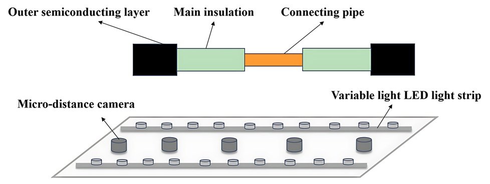
As the defects are relatively subtle compared to the cable as a whole. Using a single camera for wide-angle shooting not only loses many details, but also causes cable imaging distortion. Therefore, a macro camera array of cable intermediate joint surface image acquisition device is used, as shown in Figure 1. After the acquisition of segmented images, the SIFT algorithm is used to stitch them together to obtain a complete image of the cable middle joint.
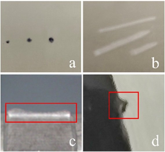
Subject to the construction techniques of the construction personnel of the good and bad, in the process of making cable joints, it is easy to cause the following four types of typical construction defects: if the main insulation is not polished, it will cause the main insulation surface stains, as shown in Figure 2(a); in the stripping of the outer semiconducting layer, if the knife is not used in a standardized manner, it is easy to cause scratches on the surface of the main insulation defects, as shown in Figure 2(b); connecting the tube crimped polished after processing is not standardized, it will make the connection tube on the existence of metal burrs, that is, crimp tube burr defects, as shown in Figure 2(c); Finally, due to peeling and cutting is not standardized, easy to cause the outer semiconducting layer and the main insulation peeling defects are not flush, as shown in Figure 2(d).
In this paper, based on the Scale-Invariant Feature Transform (SIFT) algorithm, a robust image stitching method is constructed for the geometrical and textural characteristics of the segmented images of cable joints. As the surface of cable joints often has local deformation, uneven illumination and different shooting angles, the traditional image alignment method is easily affected by the lack of feature stability, and the SIFT algorithm can effectively solve the above challenges and realize high-precision image splicing through multi-scale feature extraction and descriptor construction. The algorithm process in this paper mainly includes four core links: scale space construction, feature point accurate localization, gradient direction histogram descriptor generation, and image alignment and fusion based on feature matching [14], [15].
A Gaussian pyramid is established by Gaussian blurring the image to varying degrees and this is used to extract feature points with scale invariance, the 2D Gaussian function is defined as shown in Eq. (1): \[\label{GrindEQ__1_} G(x,y,\sigma )=\frac{1}{2\pi \sigma ^{2} } e^{\frac{-(x^{2} +y^{2} )}{2\sigma ^{2} } } , \tag{1}\] \(G(x,y,\sigma )\) is a Gaussian function and \(\sigma\) is a scale space factor as shown in Eq. (2): \[\label{GrindEQ__2_} \sigma \nabla ^{2} G=\frac{G(x,y,k\sigma )-G(x,y,\sigma )}{k\sigma -\sigma } , \tag{2}\] where \(G(x,y,\sigma )\) denotes the Gaussian kernel; k is a positive constant.
Candidate feature points are localized by 3D polar detection in Difference of Gaussian (DoG) space\(D(x,y,\sigma )=L(x,y,k\sigma )-L(x,y,\sigma )\) .Each pixel needs to be compared with 26 points in the adjacent scale and spatial neighborhood to filter out the extreme points with significant contrast. For the possible noise interference in the cable image, 3D quadratic function fitting is used for localization: \[\label{GrindEQ__3_} \hat{x}=-\frac{\partial ^{2} D^{-1} }{\partial x^{2} } \frac{\partial D}{\partial x} . \tag{3}\]
The edge response points are also eliminated using the trace to determinant ratio of the Hessian matrix. It is verified that this method can reduce the pseudo-feature points in the cable joint image significantly and improve the accuracy of subsequent matching.
After the above steps, the algorithm obtains stable feature point coordinates possessing scale invariance. By calculating the gradient modes and gradient angles around the image feature points, the pixel gradient magnitude m(x y) and direction \(\theta\)(x y) are computed within the feature point neighborhood (16\(\mathrm{\times}\)16 window), and the corresponding direction is assigned to each feature point to achieve rotational invariance. \[\begin{aligned} \label{GrindEQ__4_} \begin{cases} m(x,y)=&\sqrt{I_{x} (x,y)^{2} +I_{y} (x,y)^{2} } , \\ \theta (x,y)=&\arctan \left(\frac{I_{y} (x,y)}{I_{x} (x,y)} \right), \end{cases} \end{aligned} \tag{4}\] where \(Ix(x,y)\) and \(I{\rm y}(x,y)\) are the gradients of the image in the x and y directions, respectively. The rotational invariance is formed by counting the principal directions by Gaussian-weighted histograms (more than 80% of the peaks are retained in multiple directions). The feature region is divided into 4\(\mathrm{\times}\)4 sub-blocks, and 8-direction gradient histograms are computed for each block, ultimately generating a 128-dimensional feature vector. By computing the gradient magnitude and direction, SIFT can generate a direction calibration for each feature point and use that direction as the datum for the feature point descriptor, making the descriptor invariant to rotation.
After the feature points are localized and described, the SIFT algorithm implements image stitching by feature point matching. For two images \(I_{1}\) and \(I_{2}\), SIFT matches the feature points by calculating the similarity between the descriptors. Let \(d_{1}\) and \(d_{2}\) be the descriptors of two feature points, then their matching is usually measured using Euclidean distance: \[\label{GrindEQ__5_} {\rm dist}(d_{1} ,d_{2} )=\parallel d_{1} -d_{2} \parallel . \tag{5}\]
In this way, SIFT is able to compute the best matching feature point pairs between images. To further improve the accuracy of the matching, SIFT uses Lowe’s ratio test to eliminate false matches: \[\label{GrindEQ__6_} \frac{{\rm dist}(d_{1} ,d_{2} )}{{\rm dist}(d_{1} ,d_{3} )} <\tau , \tag{6}\] where \(d_{1}\) is the descriptor of the current feature point, \(d_{2}\) and \(d_{3}\) are the descriptors of its nearest and second nearest neighbors, respectively, and \(\tau\) is the ratio threshold, which usually takes the value of 0.8. This strategy effectively reduces the probability of false matching.
After the image feature point matching is completed, the SIFT algorithm uses the RANSAC algorithm for geometric transformation estimation. RANSAC obtains the final transformation matrix \(H\) by randomly selecting the matched point pairs and calculating the transformation matrix, and iteratively optimizes it to ensure geometric alignment during the splicing process. By calculating the transform matrix, SIFT is able to realize seamless splicing of cable intermediate joint images and generate high-quality spliced images.
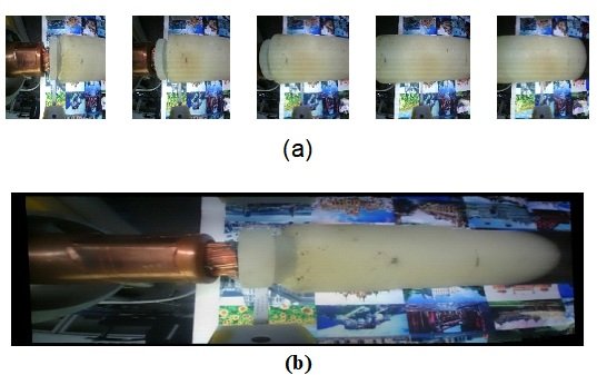
The splicing effect is shown in Figure 3(a) and Figure 3(b) below:
YOLO11, as the latest generation model of YOLO (You Only Look Once) series, realizes a breakthrough in the balance of accuracy and speed in the field of real-time target detection. Its core innovation lies in the introduction of C2PSA module and C3k2 module, which significantly improves the detection performance in complex scenes through multi-scale feature fusion and efficient attention mechanism, and its model architecture is shown in Figure 4. The following is a detailed description of the model architecture in terms of its core modules, optimization mechanism and performance comparison.
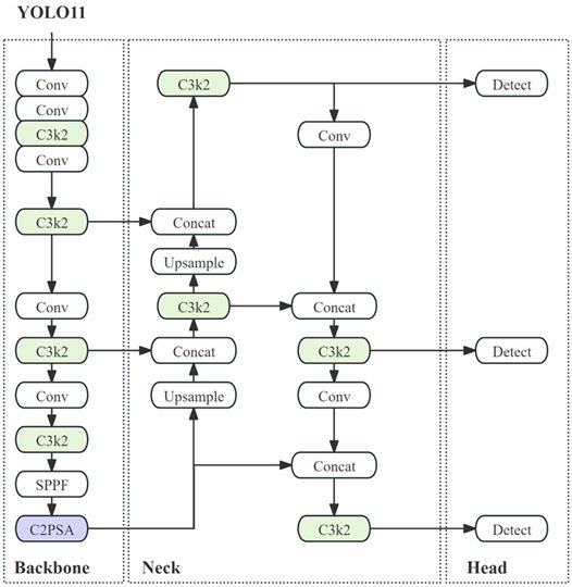
The backbone network of YOLO11 is based on an improved cross-stage partial (CSP) structure, which focuses on optimizing the feature extraction efficiency and information transfer capability. While the traditional CSP module reduces redundant computations by splitting the feature map, YOLO11 further introduces the C3k2 module with a compact 3\(\mathrm{\times}\)3 convolutional kernel stacking structure, which reduces the computation amount while retaining the deep feature expression capability.
The neck of YOLO11 employs the Spatial Pyramid Fast Pooling (SPFF) module to enhance small target detection through multi-scale pooling operations. SPFF combines pooling kernels of different sizes (e.g., 5\(\mathrm{\times}\)5, 9\(\mathrm{\times}\)9, and 13\(\mathrm{\times}\)13) to perform parallel pooling on the input feature maps, followed by multi-resolution feature splicing and dimensionality reduction through 1\(\mathrm{\times}\)1 convolution. This design effectively captures the contextual information of targets of different sizes in the image and solves the problem of excessive computation of traditional pyramid pooling. Further, YOLO11 introduces the C2PSA (Cross-Stage Partial Pyramid Slice Attention) module in the neck, which is improved based on the SE (Squeeze-and-Excitation) attention mechanism.C2PSA splits the feature map into multi-scale subregions by pyramid slice operation and applies channel attention weights on each sub-region to dynamically enhance the response of key regions.
The detection head of YOLO11 continues the multi-scale prediction framework of YOLOv8, but improves the decoupling design of the classification and regression branches. The details are as follows:
Classification branch: depth separable convolution (DWConv) is used instead of traditional convolution, and the number of parameters is significantly reduced.
Regression branch: a dynamic anchor frame mechanism is introduced to automatically adjust the initial anchor frame size according to the training data distribution, reducing the manual design bias.
In terms of training strategy, YOLO11 adopts progressive learning rate scheduling with Mosaic Augmentation to mitigate model overfitting by dynamically adjusting the data augmentation strength and learning rate curve. In addition, its loss function integrates CIoU (Complete Intersection over Union) and Focal Loss to optimize the bounding box localization and category imbalance problems.
In the cable joint construction defect detection, due to the object to be detected, such as the main insulation stains and scratches and crimp tube burrs and other defects with the cable intermediate joints as a whole compared to the more subtle, that is, belongs to a small target range of detection objects. In addition, the main insulation stains and semiconducting layer peeling defects in the actual joint production process by the construction personnel craft uncontrollable factors, resulting in its shape variable, as well as defects scale changes, and thus the robustness of the detection is greatly affected. Finally, due to the unavoidable noise and brightness of the capture device, some defects may have blurred edges in the image presentation, which further increases the difficulty of detection.
To address the above problems, a DLP2-YOLO11s network model is proposed, the structure of which is shown in Figure 5.
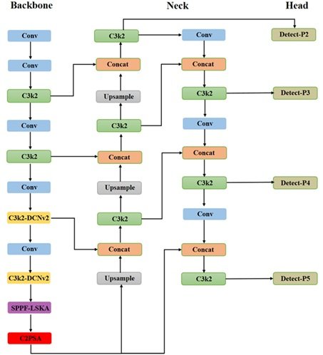
The DCNv2 module is first introduced in the key layers of the Backbone section to enhance the adaptability to irregularly shaped defects. In the P4/16 (layer 6) and P5/32 (layer 8) stages, the standard convolution is replaced by the C3k2_DCNv2 module, which dynamically adjusts the sensory field through deformable convolution to capture the irregular boundary information of the defects. The offset learning mechanism of DCNv2 enables the model to better adapt to the deformation characteristics of the construction defects (e.g., the random morphology of the main insulation stains, the uneven irregularity of the stripped semiconducting layer, the irregularity of the edge), and improves the robustness of different morphology detection. edges), improving the robustness of different morphology detection. In addition, the SPPF_LSKA module (layer 9) is introduced to expand the receptive field through the decomposed large kernel convolution, which is combined with the channel attention to screen the critical region, effectively suppressing the noise interference, strengthening the edge response of low-contrast defects (e.g., light-colored scratches), and solving the leakage detection problem of fuzzy defects.
A new P2/4 detection layer is added to the Neck section to construct a four-layer (P2-P5) feature pyramid. The feature map resolution of the P3 layer is improved from 1/8 to 1/4 (160\(\mathrm{\times}\)160) by up-sampling the branch, and connected across the layers with the original P2 features in the shallow Backbone layer. This method takes full advantage of the high spatial resolution of the shallow features to significantly improve the localization accuracy of small target defects (e.g., crimp tube burrs with width \(\mathrm{<}\)20px). In addition, in the downsampling branch, P2-P5 cross-layer feature fusion is realized through Conv layer downsampling and Concat operation. This makes the high-level semantic information (e.g., the overall shape of the stain) complementary to the underlying details (e.g., the localized texture of the scratch), and enhances the model’s joint perception of multi-scale defects (e.g., the large-scale anomaly of the semiconducting layer peeling misalignment and the small-scale spots of the stain). Finally, all cross-layer connections use C3k2 modules to reduce parameter redundancy through deeply separable convolution, which guarantees the efficiency of multi-scale information fusion while avoiding the risk of overfitting due to feature dimension inflation.
In the Head section, the new P2 inspection head and channel count redesign solve the problem of missing small defects. The new P2 head is based on 1/4 scale feature map (160\(\mathrm{\times}\)160 resolution), its pixel density is 4 times higher than the traditional P3 head (80\(\mathrm{\times}\)80 resolution), which is able to effectively capture the small defects on the surface of cable joints. Finally, according to the defect scale distribution characteristics, the asymmetric design of the number of channels of the detection head is carried out: 128 channels are used in the P2 detection head, focusing on detailed feature extraction; 1024 channels are used in the P5 detection head, focusing on the global semantic information. This strategy reduces the redundancy of deep features while ensuring that the computational resource share of small target detection is increased, realizing the balance between detection efficiency and accuracy.
Step 1: Deformable convolution C3k2-DCNv2
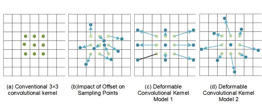
In the traditional architecture of neural networks, the sampling points of the convolutional kernel usually follow a uniform distribution pattern and their shapes are fixed. This design makes the convolutional layer limited to sampling operations at preset locations when processing the input feature maps, which in turn limits the model’s ability to recognize diverse features. To address this problem, literature [16], [17] proposes a deformable convolutional network that optimizes the conventional convolution process by introducing a convolution kernel that can adaptively adjust its shape and the location of sampling points. This improvement enables the model to adaptively obtain receptive fields of different sizes and shapes according to the feature maps of different regions, thus dealing with the spatial variations of the target object more efficiently.
In DCNv2, the sampling position of each convolutional kernel is obtained by adaptive learning through the training process and can be flexibly adjusted according to the characteristics of the input image, so as to capture the non-rigid deformation of the target object and improve the model’s perceptual ability. In addition, DCNv2 introduces offsets, which are used to characterize the offsets of the sampling points relative to the initial positions. These displacement values are iteratively optimized through the training process and used to further adjust the actual range of the convolution kernel [18].
As shown in Figure 6, where (a) demonstrates the sampling point distribution of a regular convolutional kernel, while (b), (c), and (d) are the sampling point distributions of a deformable convolutional kernel. The two types of convolutional kernels are of the same size, but there is a significant difference in the sampling point locations.
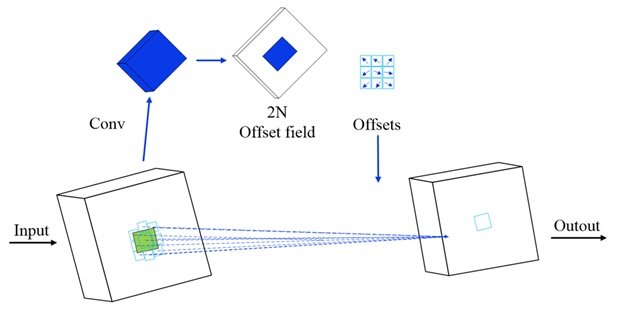
Figure 7 illustrates the workflow of the deformable convolutional kernel. The generation of offsets is accomplished through an independent network branch, which performs a convolution operation on the input feature map to produce an offset feature map containing 2N channels. The pixel-level offsets are iteratively optimized by a bilinear interpolation backpropagation algorithm, where the offset parameters are typically expressed as floating-point values. The input feature maps are convolved with the optimized offsets to finally generate the target output feature maps.
The eigenvalue output formula for deformable convolutional kernel sampling is: \[\label{GrindEQ__7_} y(p)=\mathop{\sum }\limits_{k=1}^{K} w_{k} \cdot x(p+p_{k} +{\rm \Delta }p_{k} )\cdot {\rm \Delta }m_{k} , \tag{7}\] where the output feature map \(y\left(p\right)\) is generated from the input feature map \(x\) by a convolution operation, where \(w_k\) is defined as the \(k\)-position convolution kernel weight, p denotes the feature map sampling centroid coordinates, and \(p_k\) is a preset offset. \(\mathrm{\Delta }p_k\) characterizes the dynamic offset with respect to the center point p, which is equivalent to the standard convolution kernel when \(\mathrm{\Delta }p_k\)=0. \(\mathrm{\Delta }m_k\) is the learnable weight in the interval [0, 1], which is set to zero for fixed sampling points (e.g., boundary regions) to enhance the flexibility of the convolution kernel deformation.
The traditional YOLO model has the problem of accuracy attenuation when detecting small-scale and densely distributed targets. With the introduction of deformable convolution, the convolution layer is able to dynamically adjust the sampling region and enhance the small target characterization ability through multi-dimensional feature acquisition. This mechanism effectively improves the detection accuracy of dense, small-scale and partially occluded targets, and significantly improves the robustness and overall performance of the model. Based on this, this study replaces the C3k2 module of the Backbone network with the DCNv2 convolutional structure, and strengthens the feature learning ability of the construction defects of cable joints through the deformable sampling mechanism, so as to optimize the performance of small target detection.
Step 2: SPPF-LSKA
Based on the structure of the Space Pyramid Pooling (SPP) module, the Spatial Pyramid Pooling-Fast (SPPF) module in the benchmark model is enhanced. The improved module adopts a three-stage tandem pooling layer structure to realize multi-scale fusion through feature splicing, which ensures the fusion effect and improves the computational efficiency at the same time. Compared with the traditional SPP module, its computational complexity is reduced, its inference speed is accelerated, and it supports adaptive processing of dynamic size input features. However, there are obvious limitations in the structure’s ability to capture fine-grained features. Although the continuous pooling process can compress the parameter scale, it leads to the loss of pixel-level detail information, which contradicts the accuracy requirements of the detection task. For the feature extraction needs in complex scenes, this study combines the LSKA attention mechanism with the SPPF module, as shown in Figure 8, to strengthen the key feature selection through attention guidance.
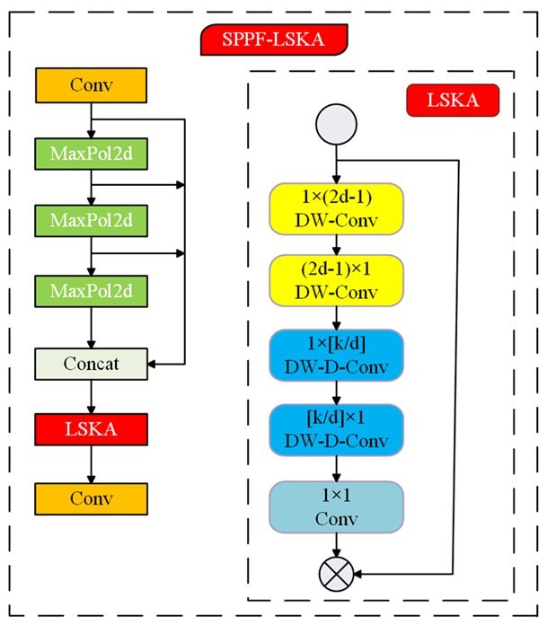
LSKA uses a separable convolutional kernel design to extract spatial dimensional information of the feature map by horizontal/vertical convolutional decomposition, respectively [19], [20]. This stage generates a primary attention heat map to guide the network to focus on image saliency regions. Subsequently, multi-level spatial expansion convolution is employed to capture multi-scale contextual information through a differentiated sense field expansion strategy. And the effective sensory field area is enlarged without significantly increasing the number of parameters. The spatial dimension decoupling operation enhances the ability to model the image geometry and makes the feature representation directionally sensitive. Finally, cross-channel feature fusion is achieved by 1 convolutional layer to generate the optimized attention map. The original feature map is multiplied with the attention map, a process that applies the attention mechanism. This mechanism enables the feature map elements to be dynamically adjusted according to the attention weights, highlighting important features and suppressing non-important features. LSKA combines the separable large kernel convolution and spatial expansion strategies to construct a multi-scale attention guidance mechanism, which enhances the network’s attention to the important features of the defects, and thus improves the detection performance of the model. Eqs. (8)-(11) completely define the mathematical expression of LSKA, where the operator \(\mathrm{\ast}\) denotes the standard convolution operation and \(\mathrm{\otimes}\) represents the element-level product operation [21]. \[\label{GrindEQ__8_} x^{c} ={\mathop{\sum }\limits_{H,W}} W_{(2d-1)\times 1}^{C} *\left({\mathop{\sum }\limits_{H,W}} W_{1\times (2d-1)}^{C} *F^{C} \right) , \tag{8}\] \[\label{GrindEQ__9_} Z^{C} ={\mathop{\sum }\limits_{H,W}} W_{\left[\frac{k}{d} \right]\times 1}^{C} \mathrm{\star }\left({\mathop{\sum }\limits_{H,W}} W_{1\times \left[\frac{k}{d} \right]}^{C} X^{C} \right) , \tag{9}\] \[\label{GrindEQ__10_} A^{C} =W_{1\times 1} \mathrm{\star }Z^{C} , \tag{10}\] \[\label{GrindEQ__11_} T^{C} =A^{C} \otimes F^{C} , \tag{11}\] where Z\({}^{C}\) represents the output of the deep convolution, which is obtained by a convolution kernel of size k\(\mathrm{\times}\)k performing a convolution operation with the input feature map. Each channel C in the feature map F performs a convolution operation with the corresponding channel in the convolution kernel W. The output T\({}^{C}\) of the LSKA module is generated by the Hadamard product operation of the attention map A\({}^{C}\) with the input feature map F\({}^{C}\). This improvement measure significantly enhances the characterization capability of the backbone feature extraction network and strengthens the recognition accuracy of the target object, thus improving the overall detection performance.
Step 3: Add P2 small target detection layer
In the target detection task, the model needs to deal with targets of different scales at the same time, and small target detection has always been a difficult task in the detection task due to its sparse feature information and high position sensitivity.YOLO11 extracts feature maps (P1-P5) of different scales by constructing a Feature Pyramid Network (FPN), in which the P2 feature map’s The resolution is 1/4 of the original image, which has higher spatial resolution and richer detail information, and is especially suitable for detecting small-scale targets. However, the traditional YOLO series models usually use only P3 (1/8 resolution) as the minimum detection layer, which leads to insufficient positional description capability for small targets. To solve this problem, this study introduces a P2-level target detection layer in the detection head (Head) of YOLO11 and combines it with the Path Aggregation Network (PANet).
First, the P2 detection layer fuses the P3 feature maps with the P2 feature maps across scales through an up-sampling operation to form a high-resolution feature map (P2/4). This design makes full use of the high-resolution property of the P2 feature map, which enhances the model’s sensitivity to and ability to accurately describe the location of small targets. At the same time, the P3 feature map is spliced with the P2 feature map through the Concat operation, which realizes the dynamic fusion of the underlying high-resolution features with the mid-level semantic features, and further enhances the richness of feature expression. In addition, the P2 level target detection layer adopts the lightweight C3k2 module for feature reconstruction, whose core consists of 3\(\mathrm{\times}\)3 convolution and residual concatenation, which enhances the model’s detection performance for small targets while maintaining computational efficiency.
By introducing the P2 small target detection layer, YOLO11 is able to utilize the position information in the high-resolution feature maps more effectively, which significantly improves the detection accuracy of small targets.
The experiments in this paper are based on the Windows operating system, using Python3.10-based Pytorch1.30 to build deep learning models. For model training, NVIDIA GEForce RTX 4060 GPU is used as the model training platform, and CUDA11.7 is used to accelerate the GPU. The parameter settings of the deep learning model are shown in Table 1.
| parameters | setting | parameters | setting |
|---|---|---|---|
| Number of categories | 4 | batch size | 16 |
| learning rate | 0.01 | training rounds | 300 |
| Image input high | 640 | optimizer | SGD |
| Image input high | 640 | Workers | 4 |
In view of the lack of public benchmark datasets for cable joint construction defects, this study constructs samples of four types of typical construction defects based on actual engineering scenarios. A special dataset containing 850 defect samples is constructed by building a dedicated cable joint image acquisition device for segmented image acquisition, combining a standardized preprocessing process with an image alignment technique based on a scale-invariant feature transformation algorithm. In order to improve the generalization ability of the model, this study implements data enhancement strategies that include geometric transformation, Gaussian noise injection, and chromaticity space random transformation, extends the sample size to 2550 images, and strictly follows the ratio of 8:1:1 to divide the training, validation, and test sets.
In order to evaluate the improvement effect of YOLO11 in this paper, the improved model is evaluated in terms of the following types of metrics: precision , recall , mean average precision (mAP ). \[\label{GrindEQ__12_} P=\frac{TP}{TP+FP}, \tag{12}\] \[\label{GrindEQ__13_} R^{} =\frac{TP}{TP+FN} , \tag{13}\] \[\label{GrindEQ__14_} AP=\smallint _{0}^{1} P\left(r\right){\rm d}r , \tag{14}\] \[\label{GrindEQ__15_} mAP=\frac{1}{n} \mathop{\sum }\limits_{i=1}^{n} AP_{i} , \tag{15}\] where TP denotes the number of correctly identified positive category samples, TN denotes the number of correctly identified negative category samples, FN denotes the number of unidentified positive category samples, and FP denotes the number of incorrectly categorized negative category samples. p denotes the proportion of predicted positive samples that are actually positive, and R denotes the proportion of actual positive samples that are correctly predicted. the AP value was obtained by calculating the area under the P-R curve. ap denotes the average precision of a single category, mAP denotes the average precision of all categories, and n denotes the total number of categories. The mAP@0.5 is defined as the average precision at an IOU threshold of 0.5, and mAP@0.5:0.95 is defined as the average precision over the range of IOU thresholds from 0.5 to 0.95 (in steps of 0.05).
Step 1: Ablation experiment
In order to verify the effectiveness of the proposed three improved algorithms on the optimization of the YOLO11 algorithm, ablation experiments were carried out under the strict control of the consistency of the model parameters, and the effects of the three improved algorithms on the detection performance of the model are shown in Table 2:
| DCNv2 | SPPF-LSKA | P2 | P/% | R% | mAP@0.5/% | GFLOPs | Params/\(\mathrm{\times}\)106 |
|---|---|---|---|---|---|---|---|
| — | — | — | 76.2 | 47.2 | 53.7 | 6.4 | 2.59 |
| \(\mathrm{\sqrt{}}\) | — | — | 74 | 49.7 | 56 | 6.4 | 2.63 |
| — | \(\mathrm{\sqrt{}}\) | — | 73.3 | 49.6 | 55.1 | 6.7 | 2.86 |
| — | — | \(\mathrm{\sqrt{}}\) | 81 | 61.4 | 69 | 10.5 | 2.67 |
| \(\mathrm{\sqrt{}}\) | \(\mathrm{\sqrt{}}\) | — | 74.8 | 46.5 | 54.2 | 6.6 | 2.91 |
| \(\mathrm{\sqrt{}}\) | — | \(\mathrm{\sqrt{}}\) | 76.5 | 58 | 65.7 | 10.8 | 2.95 |
| — | \(\mathrm{\sqrt{}}\) | \(\mathrm{\sqrt{}}\) | 78.9 | 62.5 | 69.1 | 11.1 | 3.17 |
| \(\mathrm{\sqrt{}}\) | \(\mathrm{\sqrt{}}\) | \(\mathrm{\sqrt{}}\) | 80.3 | 62.1 | 70.3 | 10.7 | 2.99 |
The experimental results show that there are significant differences in the impact of each improved algorithm module on model performance and computational efficiency, and the synergy between the modules needs to seek a balance between accuracy improvement and resource consumption.
First, when the DCNv2 module is introduced into the benchmark model alone, the number of model parameters (Params) is slightly increased from 2.59 \(\mathrm{\times}\) 10\(^6\) to 2.63 \(\mathrm{\times}\) 10\(^6\) (+1.5%), while the computational volume (GFLOPs) remains unchanged at 6.4, at which time the recall (R) is improved by 2.5% to 49.7% and the mAP@0.5 increases by 2.3% to 56.0%. This phenomenon indicates that DCNv2 enhances feature representation through the geometric adaptive property of deformable convolutional kernel, and its parameter increment mainly comes from the lightweight design of the offset prediction branch, which does not significantly increase the computational load. However, the accuracy (P) decreases by 2.2% to 74.0%, which may be attributed to the local feature perturbation introduced by dynamic convolution, resulting in a shift in classification confidence.
Second, when the SPPF-LSKA module is added alone, it improves the mAP@0.5 by 1.4% to 55.1% through long-range dependency modeling, but its high parameter count cost and computational complexity limit the deployment efficiency, and the accuracy decreases by 2.9% to 73.3%, which indicates that the large kernel convolution may dilute the local detailed features and lead to blurred classification boundaries.
In contrast, the introduction of the P2 small target detection layer significantly improves the model detection performance, bringing about a 15.3% jump in mAP@0.5 (to 69.0%), despite its high-resolution feature maps spiking the computational effort by 64.1% to 10.5 GFLOPs, and a slight increase in the number of parameters to 2.67 \(\mathrm{\times}\) 10\(^6\) (+3.1%). It shows that the introduction of the P2 small target detection layer has a significant effect on the improvement of construction defect detection accuracy of cable intermediate joints.
In terms of module combination optimization, the combined use of SPPF-LSKA and P2 small target detection layer achieves a parameter count of 3.17 \(\mathrm{\times}\) 10\(^6\) (+22.4%) and a computational volume of 11.1 GFLOPs (+73.4%), but the recall rate (62.5%) and mAP@0.5 (69.1%) are close to the optimal value of the three-module fully-enabled (70.3%), which suggests that the large kernel attention of the multiple scale pooling complements the high-resolution features. The all-module configuration (DCNv2+SPPF-LSKA+P2) achieves an absolute improvement of 16.6% in mAP@0.5 at the cost of 2.99\(\mathrm{\times}\)10\(^6\) (+15.4%) in the number of parameters and 10.7 GFLOPs (+67.2%) in the computation, verifying that the composite-module synergetic combinations break through the performance bottlenecks of a single module.
Step 2: Comparison experiment
In order to further validate the effect of the improved algorithm proposed in this paper on the construction defect detection of cable intermediate joints, the improved algorithm is compared with YOLO11s, YOLO11-CBAM with added CBAM attention mechanism, YOLO11-AFPNHead with added AFPN (Asymptotic Feature Pyramid Network) detector head, and YOLOv8s in the same dataset and experimental environment, YOLOv5s, YOLOv10n, and YOLOv3-tiny current mainstream target detection models for comparison. The experimental results are shown in Table 3.
| MOULD | P/% | R/% | mAP@0.5/% | GFLOPS | Parameters/106 |
|---|---|---|---|---|---|
| YOLO11s | 0.762 | 0.472 | 0.537 | 6.4 | 2.59 |
| YOLO11-CBAM | 0.753 | 0.451 | 0.525 | 6.4 | 2.64 |
| YOLO11-AFPNHead | 0.652 | 0.412 | 0.422 | 6.7 | 2.70 |
| YOLOv8s | 0.755 | 0.503 | 0.575 | 6.8 | 2.68 |
| YOLOv5s | 0.753 | 0.486 | 0.562 | 5.8 | 2.18 |
| YOLOv10n | 0.739 | 0.526 | 0.612 | 6.5 | 2.26 |
| YOLOv3-tiny | 0.663 | 0.296 | 0.366 | 14.3 | 9.52 |
| ARTICLE | 0.803 | 0.621 | 0.703 | 10.7 | 2.99 |
According to the results of the comparative experiments in Table 3, the performance of different algorithms in the task of detecting construction defects in cable intermediate joints varies significantly. The YOLO11s benchmark model, while maintaining a low computational complexity (6.4 GFLOPS) with a low number of parameters (2.59 \(\mathrm{\times}\) 10\(^6\)), only achieves a mAP@0.5 of 53.7%, which indicates that the original architecture’s capability of feature characterization for fine defects, such as insulation stains and scratches, is Insufficient. Although the number of parameters of the model introducing the CBAM attention mechanism is slightly increased to 2.64\(\mathrm{\times}\)10\(^6\), the mAP@0.5 inversely decreases to 52.5%, which speculates that the channel-spatial attention mechanism may interfere with the focusing of local defect features under complex background noise. The performance of the YOLO11-AFPNHead model with adaptive feature pyramid further deteriorates (mAP@0.5=42.2%), which verifies that the multi-scale feature fusion strategy is mismatched with the scale-distribution characteristics of the cable surface defects, and its computational cost of 6.7 GFLOPS does not result in effective performance gain.
Comparing the mainstream lightweight models, YOLOv5s and YOLOv8s have a mAP@0.5 of 56.2% and 57.5%, respectively, which is better than the benchmark YOLO11s, but its recall still struggles to cover construction defect detection.YOLOv10n achieves a mAP@0.5 of 61.2% by the structural reparametrization technique, but the imbalance between its precision rate (73.9%) and recall rate (52.6%) indicates its limitation in localizing irregular targets such as crimp tube burrs. The traditional lightweight model YOLOv3-tiny has a mAP@0.5 of only 36.6%, and the high computational cost of 14.3 GFLOPS with 9.52 \(\mathrm{\times}\) 10\(^6\) parameter count highlights the inefficiency of its architectural design.
The improved model proposed in this paper improves the mAP@0.5 to 70.3%, achieving an absolute gain of 16.6%, 12.8% and 9.1% over the benchmarks YOLO11s, YOLOv8s and YOLOv10n, respectively. Despite the increase in the number of model parameters to 2.99\(\mathrm{\times}\)10\(^6\) (15.4% increase over YOLO11s) and the computational cost to 10.7 GFLOPS (+67.2%), its unit computational efficiency (mAP@0.5/GFLOPS=6.57%) is still significantly better than YOLOv3-tiny (2.56%) and YOLO11-AFPNHead (6.30%). The experimental results show that the algorithm in this paper can meet the demand for high-precision real-time detection of construction defects in cable intermediate joints by combining the three types of improved modules to achieve a better trade-off between detection accuracy and computational resource consumption..
moduIn light of the current lack of high-precision methods for identifying defects in various components, this paper proposes a defect detection method that integrates the U-Net algorithm with the Canny algorithm. The U-Net algorithm accurately segments these components, while the Canny algorithm effectively extracts their edge information, achieving an accuracy rate of over 90%. The proposed algorithm enhances the capability to identify different types of defects, thereby improving the reliability of cable operations prior to their deployment.
It is evident that utilizing specific algorithms tailored to different types of defects can enhance the accuracy of defect recognition. The method introduced in this paper efficiently detects defects such as scratches and stains on the main insulation, burrs on the crimping tube, uneven cuts in the semi-conductive layer, and irregular cuts along the edges of the main insulation, thereby providing reliable measures for managing and controlling the quality of cable construction technology.
In this study, an intelligent detection algorithm integrating image processing and improved YOLOv11 is proposed for the difficult problem of multi-scale small target detection in the construction defect detection of intermediate joints of high-voltage cables.
First, based on the multi-camera cooperative acquisition device and SIFT feature adaptive alignment algorithm, the panoramic splicing of cable joints is realized, which effectively solves the defect leakage detection problem caused by single-view imaging.
Secondly, the deformable convolutional DCNv2 module is introduced at the algorithmic level to enhance the model’s dynamic deformation modeling capability for irregular targets such as semiconducting layer peeling irregularities, the LSKA large kernel attention mechanism is used to enhance global contextual awareness, and the feature expression of tiny defects such as main insulation stains, scratches, crimp tube burrs, and so on, is strengthened by the P2 small target detection layer.
Experiments show that the improved model achieves 80.3% detection accuracy and 70.3% mAP@0.5 on the self-constructed cable defects dataset, which is 4.1% and 16.6% higher than the benchmark YOLO11s, respectively, and the recall rate of low-contrast defects reaches 62.1%, which is significantly better than the existing mainstream lightweight models (YOLOv8s/YOLOv10n). Although the number of model parameters and computational complexity increase to 2.99\(\mathrm{\times}\)10\(^6\) and 10.7 GFLOPS, respectively, its unit computational efficiency (mAP@0.5/GFLOPS=6.57%) is still better than the comparison algorithm, which verifies the superiority of the improved model in terms of precision-efficiency trade-off. The results provide a reliable solution for cable joint construction quality assessment in power systems. Future research will further optimize the highly accurate real-time identification of subtle defects under panoramic images to promote the in-depth application of intelligent inspection technology in power equipment inspection.
The authors declare that the research was conducted in the absence of any commercial or financial relationships that could be construed as a potential conflict of interest.
All claims expressed in this article are solely those of the authors and do not necessarily represent those of their affiliated organizations, or those of the publisher, the editor and the reviewers. Any statements, claims, performances and results are not guaranteed or endorsed by the publisher.
This work was supported in part by Science and Technology Projects of State Grid Corporation of China (5500-202255402A-2-0-ZN).